Neural Networks

2/15/2024

Ample material adapted from http://neuralnetworksanddeeplearning.com

print view

%%html
<script src="https://bits.csb.pitt.edu/preamble.js"></script>

Perceptron

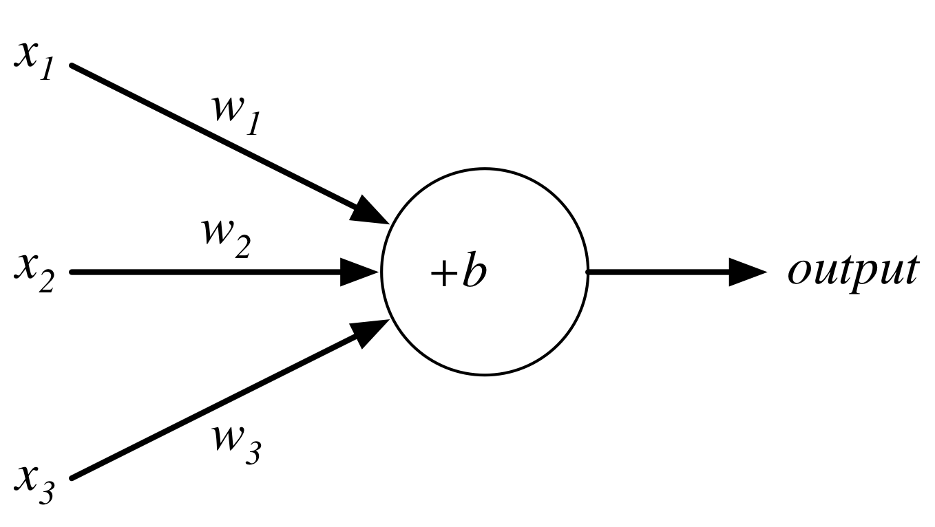
$$output = \begin{cases} 0 \text{ if } w\cdot x + b \le 0 \\ 1 \text{ if } w\cdot x + b > 0 \end{cases}$$

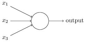
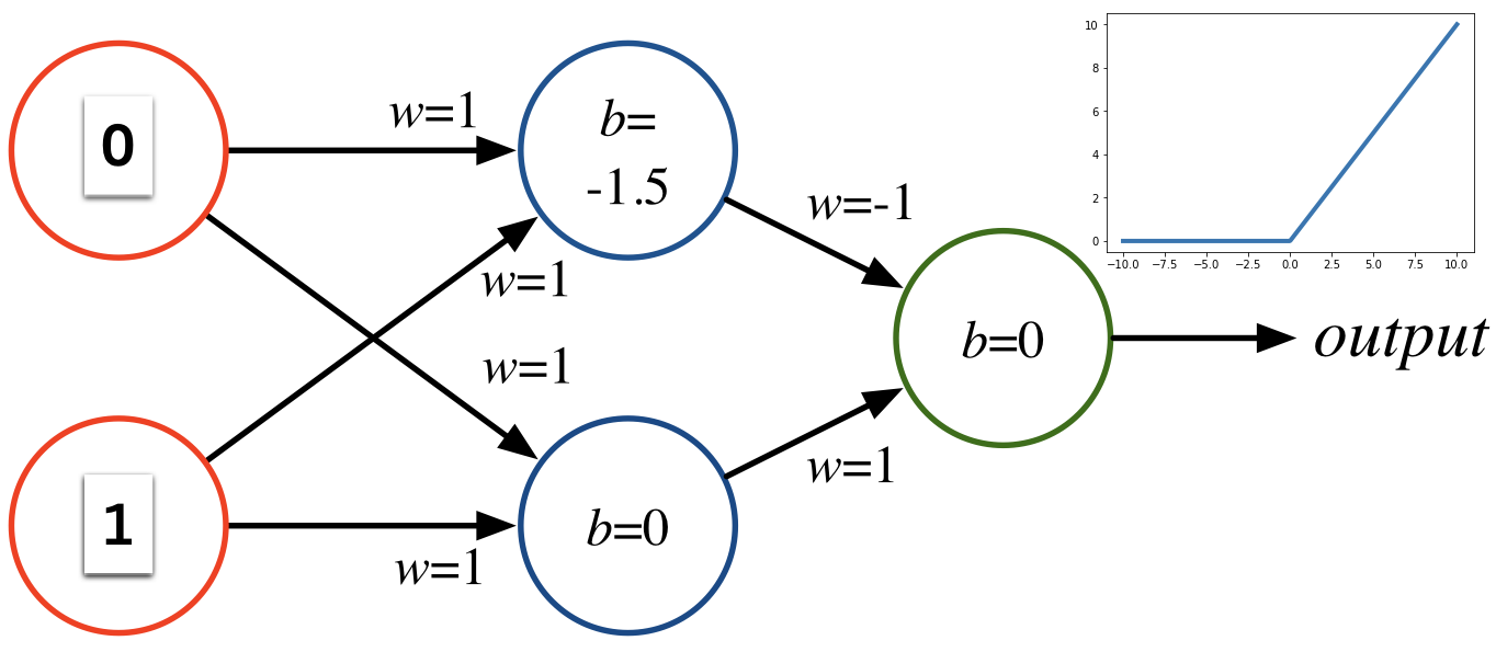
Perceptron

Consider the following perceptron:

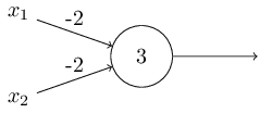
If $x$ takes on only binary values, what are the possible outputs?

%%html
<div id="nand" style="width: 500px"></div>
<script>

    var divid = '#nand';
	jQuery(divid).asker({
	    id: divid,
	    question: "What are the corresponding outputs for x = [0,0],[0,1],[1,0], and [1,1]?",
		answers: ["0,0,0,0","0,1,1,0","0,0,0,1","0,1,1,1","1,1,1,0"],
        server: "https://bits.csb.pitt.edu/asker.js/example/asker.cgi",
		charter: chartmaker})
    
$(".jp-InputArea .o:contains(html)").closest('.jp-InputArea').hide();


</script>

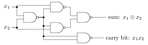
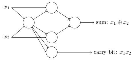
Perceptron

We can implement a NAND gate with a perceptron.. so we can basically compute anything with enough perceptrons.

http://www.cse.chalmers.se/~coquand/AUTOMATA/mcp.pdf

Neurons

Instead of a binary output, we set the output to the result of an activation function $\sigma$

$$output = \sigma(w\cdot x + b)$$

Activation Functions: Step (Perceptron)

plt.plot(x, x > 0,linewidth=1,clip_on=False);
plt.hlines(xmin=-10,xmax=0,y=0,linewidth=3,color='b')
plt.hlines(xmin=0,xmax=10,y=1,linewidth=3,color='b');

Activation Functions: Sigmoid (Logistic)

plt.plot(x, 1/(1+np.exp(-x)),linewidth=4,clip_on=False);

plt.plot(x, 1/(1+np.exp(-2*x)),linewidth=2,clip_on=False);
plt.plot(x, 1/(1+np.exp(-.5*x)),linewidth=2,clip_on=False);

Activation Functions: tanh

plt.plot([-10,10],[0,0],'k--')
plt.plot(x, np.tanh(x),linewidth=4,clip_on=False);

Activation Functions: ReLU

Rectified Linear Unit: $\sigma(z) = \max(0,z)$

plt.plot(x,x*(x > 0),clip_on=False,linewidth=4);

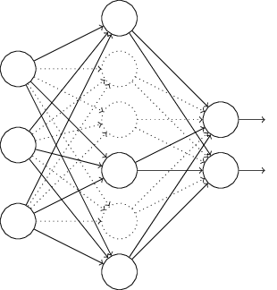
Networks

Terminology alert: networks of neurons are sometimes called multilayer perceptrons, despite not using the step function.

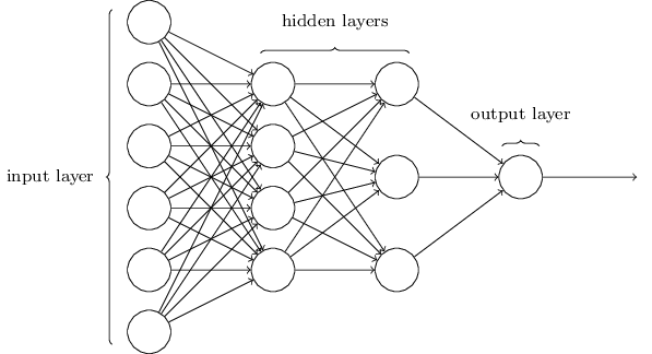
Networks

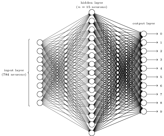The number of input neurons corresponds to the number of features.

The number of output neurons corresponds to the number of label classes. For binary classification, it is common to have two output nodes.

Layers are typically fully connected.

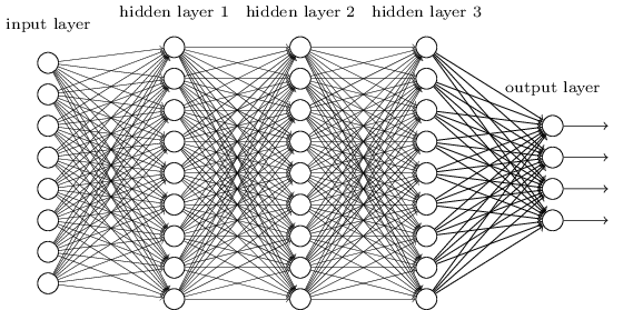
Neural Networks

The universal approximation theorem says that, if some reasonable assumptions are made, a feedforward neural network with a finite number of nodes can approximate any continuous function to within a given error $\epsilon$ over a bounded input domain.

The theorem says nothing about the design (number of nodes/layers) of such a network.

The theorem says nothing about the learnability of the weights of such a network.

These are open theoretical questions.

Given a network design, how are we going to learn weights for the neurons?

Stochastic Gradient Descent

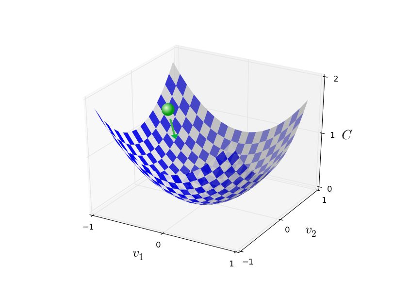
Randomly select $m$ training examples $X_j$ and compute the gradient of the loss function ($L$). Each random selection of $m$ examples is called a batch. Update weights and biases with a given learning rate $\eta$. $$ w_k' = w_k-\frac{\eta}{m}\sum_j^m \frac{\partial L_{X_j}}{\partial w_k}$$ $$b_l' = b_l-\frac{\eta}{m} \sum_j^m \frac{\partial L_{X_j}}{\partial b_l} $$

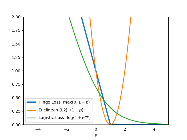
Common loss functions: logistic, hinge, cross entropy, euclidean

%%html
<div id="bpopt" style="width: 500px"></div>
<script>
$('head').append('<link rel="stylesheet" href="https://bits.csb.pitt.edu/asker.js/themes/asker.default.css" />');

    var divid = '#bpopt';
	jQuery(divid).asker({
	    id: divid,
	    question: "Will SGD (eventually) converge to a global optimum?",
		answers: ["Yes","No","Depends"],
        server: "https://bits.csb.pitt.edu/asker.js/example/asker.cgi",
		charter: chartmaker})
    
$(".jp-InputArea .o:contains(html)").closest('.jp-InputArea').hide();


</script>

Loss Functions

x = 1 is a correct prediction

Softmax

For classification problems, we modify the activation function of the output layer to be a softmax:

$$a^N_j = \frac{e^{z^N_j}}{\sum_k e^{z^N_k}}$$

This forces the output to produce a probability distribution that sums to one across all the classes.

Softmax with a log likelihood loss also avoids vanishing gradients (trains faster).

def softmax(z):
    return np.exp(z)/np.sum(np.exp(z))

softmax([0,0,1])

array([0.21194156, 0.21194156, 0.57611688])

softmax([10,0,-2])

array([9.99948459e-01, 4.53975898e-05, 6.14389567e-06])

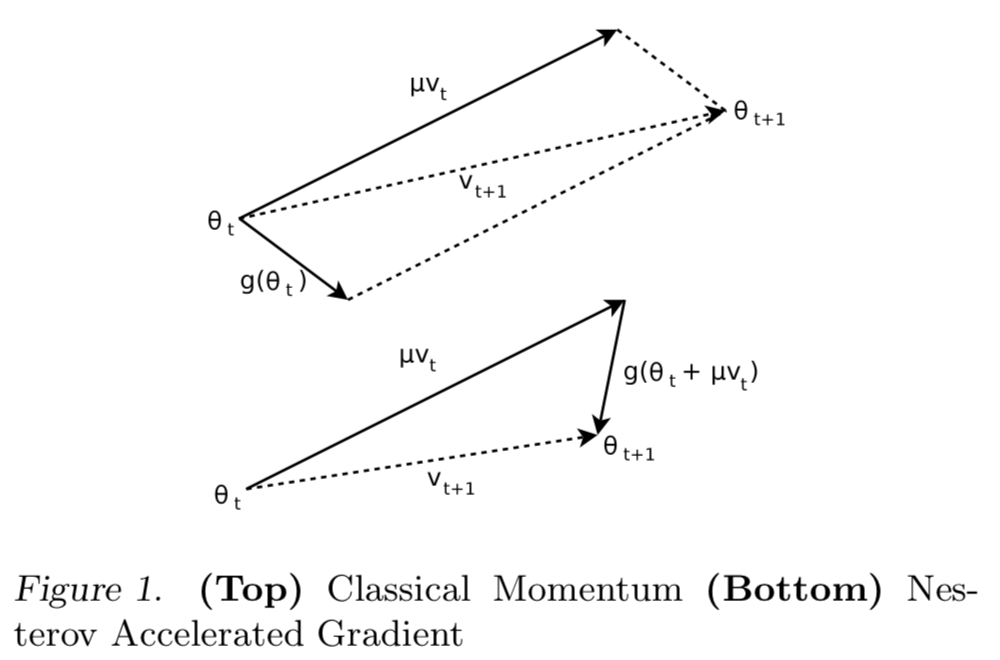
Momentum

We add momentum to our update rule by keeping track of a velocity, an accumulated history of changes. This is incorporated into our weight update using a momentum coefficient, $\mu$, (another hyper-parameter).

$$ v' = \mu v - \eta \nabla L$$ $$ w' = w+v'$$

%%html
<div id="moment" style="width: 500px"></div>
<script>

    var divid = '#moment';
	jQuery(divid).asker({
	    id: divid,
	    question: "For what value of mu does the momentum update rule reduce to SGD?",
		answers: ["0","1","0.5","None of the above"],
        server: "https://bits.csb.pitt.edu/asker.js/example/asker.cgi",
		charter: chartmaker})
    
$(".jp-InputArea .o:contains(html)").closest('.jp-InputArea').hide();


</script>

Nesterov Momentum

Keep going in along the current built-up direction, but then correct the direction.

$$ v' = \mu v - \eta \nabla L(W+\mu v)$$ $$ w' = w+v'$$

Sutskever I, Martens J, Dahl G, Hinton G. On the importance of initialization and momentum in deep learning. In International conference on machine learning 2013 Feb 13 (pp. 1139-1147).

http://www.cs.toronto.edu/~hinton/absps/momentum.pdf

from numpy import exp,arange
from pylab import meshgrid,cm,imshow,contour,clabel,colorbar,axis,title,show
import seaborn as sns
 
def plotf(f):
    plt.figure(figsize=(5,5))
    x = arange(-2.0,2.0,0.1)
    y = arange(-2.0,2.0,0.1)
    X,Y = meshgrid(x, y) # grid of point
    Z = f(X, Y) # evaluation of the function on the grid

    im = imshow(Z,origin='lower',extent=[-2,2,-2,2])
    cset = contour(Z,arange(0,2,0.5),linewidths=2,cmap=cm.Set2,extent=[-2,2,-2,2])
    clabel(cset,inline=True,fmt='%1.1f',fontsize=10)
    colorbar(im) # adding the colobar on the right

    
def plotpt(pt,grad):
    ax = plt.gca()
    plt.plot([pt[0]],[pt[1]],'o',color='white')
    d = np.array(pt)+np.array(grad)
    ax.annotate("",xy=d,xycoords='data',xytext=pt, textcoords='data', annotation_clip=False,
               arrowprops={'arrowstyle':'->','color':'white'})    

def f(x,y):
    return x**2+np.abs(0.1*y)

def g(x,y):
    return np.array([2*x,np.sign(y)*0.1])

plotf(f)
plotpt((-1,1),-g(-1,1));

def plot_grad_descent(eta):
    pt = np.array([-1,1])
    plotf(f)
    for _ in range(10):
        plotpt(pt, -eta*g(*pt))
        pt = pt - eta*g(*pt)
    plt.title("Gradient Descent ($\eta$=%.2f)"%eta)
plot_grad_descent(0.6)

def plot_cm(eta,mu):
    v = np.zeros(2); pt = np.array([-1,1]); plotf(f)
    for _ in range(10):
        v = mu*v - eta*g(*pt)
        plotpt(pt, v)
        pt = pt + v
    plt.title("Classical Momentum ($\eta$=%.2f, $\mu$=%.2f)"%(eta,mu))
plot_cm(0.6,0.9)

def plot_nesterov(eta,mu):
    v = np.zeros(2); pt = np.array([-1,1]); plotf(f)
    for _ in range(10):
        v = mu*v - eta*g(*(pt+mu*v))
        plotpt(pt, v)
        pt = pt + v
    plt.title("Nesterov Momentum ($\eta$=%.2f, $\mu$=%.2f)"%(eta,mu));
plot_nesterov(0.6,.9)

Can still screw up...

plot_nesterov(0.7,0.9)

Can make more progress with a smaller learning rate

plot_grad_descent(0.1)

plot_cm(0.1,0.9)

plot_nesterov(0.1,0.9)

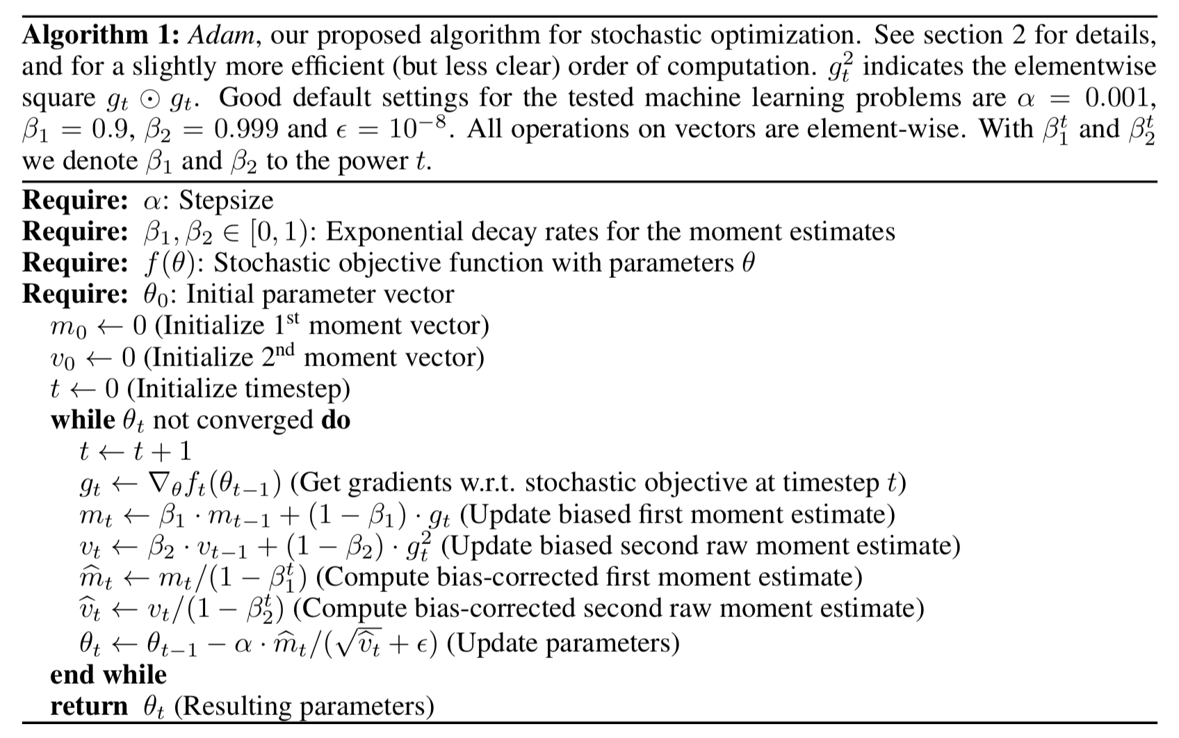
Adam

Kingma DP, Ba J. Adam: A method for stochastic optimization. arXiv preprint arXiv:1412.6980. 2014 Dec 22. https://arxiv.org/pdf/1412.6980.pdf

Backpropagation

Backpropagation is an efficient algorithm for computing the partial derivatives needed by the gradient descent update rule. For a training example $x$ and loss function $L$ in a network with $N$ layers:

1. Feedforward. For each layer $l$ compute $$a^{l} = \sigma(z^{l})$$ where $z$ is the weighted input and $a$ is the activation induced by $x$ (these are vectors representing all the nodes of layer $l$).

2. Compute output error $$\delta^{N} = \nabla_a L \odot \sigma'(z^N)$$ where $ \nabla_a L_j = \partial L / \partial a^N_j$, the gradient of the loss with respect to the output activations. $\odot$ is the elementwise product.

3. Backpropagate the error $$\delta^{l} = ((w^{l+1})^T \delta^{l+1}) \odot \sigma'(z^{l})$$

4. Calculate gradients $$\frac{\partial L}{\partial w^l_{jk}} = a^{l-1}_k \delta^l_j \text{ and } \frac{\partial L}{\partial b^l_j} = \delta^l_j$$

%%html
<div id="bpcnt" style="width: 500px"></div>
<script>

    var divid = '#bpcnt';
	jQuery(divid).asker({
	    id: divid,
	    question: "A network has 10 input nodes, two hidden layers each with 10 neurons, and 10 output neurons.  How many parameters does training have to estimate?",
		answers: ["30","100","300","330","600"],
        server: "https://bits.csb.pitt.edu/asker.js/example/asker.cgi",
		charter: chartmaker})
    
$(".jp-InputArea .o:contains(html)").closest('.jp-InputArea').hide();


</script>

Regularization

We can add L2 regularization to our loss function:

$$L = L_O + \frac{\lambda}{2n} \sum_w w^2$$

where $L_O$ is the original loss function. The gradient update rule becomes:

$$ w' = w-\eta \frac{\partial L_O}{\partial w}-\frac{\eta \lambda}{n} w $$

The $\lambda$ parameter is refered to as the weight decay.

Why is favoring smaller weights good?

Dropout Regularization

In each training iteration

1. Select a random subset of interior nodes.
2. Remove these nodes
3. Updated the weights with backpropagation
4. Restore the nodes

Makes network more robust - less sensitive to small perturbations.

Data Augmentation

More data is always better.

Getting labeled data is difficult.

So make reasonable modifications to existing data to expand the training set. For example, for images apply random small rotations/translations.

How to Scale It?

Two sources of parallelism:

1. Fine-grained parallelism. Weights in a given layer can be applied (forward pass) or updated (backward pass) in parallel using the exact same update rule but with different data.
2. Course grained parallelism. Batches of input examples can be trained in parallel (complete forward-backpass for each) and resulting weights merged (averaged).

Fine Grained Parallelism: SIMD

Single Instruction, Multiple Data

MMX, SSE, AVX, AVX2, AVX-512 etc.

Optimized math libraries (Eigen, Intel MKL, ATLAS) will use these.

Fine Grained Parallelism: GPUs

GP100 = 56 streaming multiprocessors, 3584 CUDA cores.

CUDA Programming Model

Compute Unified Device Architecture

Host (CPU) and Device (GPU) are essentiall separate computers with their own memory and compute resources.

Host tells device what to compute. Computation is performed asynchronously (not lazy).

https://en.wikipedia.org/wiki/CUDA

CUDA Programming Model

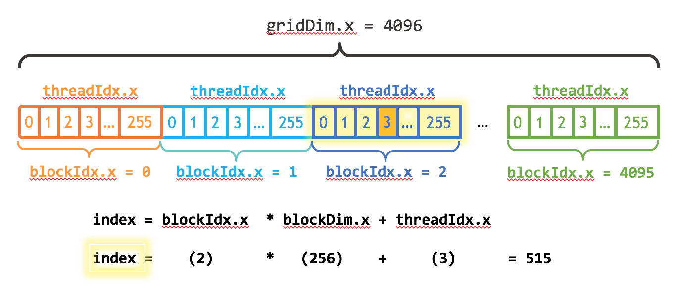
Work is divided into a grid of blocks of threads.

At most 1024 threads per a block.

Threads in the same block have shared resources exclusive to that block.

Every thread executes the same code (called a kernel).

CUDA defined variables (threadId, blockIdx) indicate which thread is running.

https://developer.nvidia.com/blog/cuda-refresher-cuda-programming-model/

CUDA Programming Model

__global__
void add(int n, float *x, float *y)
{
  int i = blockIdx.x * blockDim.x + threadIdx.x;
  if ( i < n )
    y[i] = x[i] + y[i];
}

int blockSize = 256;
int numBlocks = (N + blockSize - 1) / blockSize;
add<<<numBlocks, blockSize>>>(N, x, y);

https://developer.nvidia.com/blog/even-easier-introduction-cuda/

Python CUDA

https://numba.readthedocs.io/en/stable/cuda/overview.html

https://nvidia.github.io/cuda-python/

from numba import cuda
import numpy as np

@cuda.jit
def add(n, x, y):
    i = cuda.blockIdx.x * cuda.blockDim.x + cuda.threadIdx.x
    if i < n:
        y[i] += x[i]

n = 1000000
x = np.random.random(n); y = np.random.random(n)
blockSize = 256
numBlocks = (n+blockSize-1)//blockSize
add[numBlocks, blockSize](n,x,y)

/home/dkoes/.local/lib/python3.10/site-packages/numba/cuda/cudadrv/devicearray.py:886: NumbaPerformanceWarning: Host array used in CUDA kernel will incur copy overhead to/from device.
  warn(NumbaPerformanceWarning(msg))

Python CUDA

xc = cuda.to_device(x)
yc = cuda.to_device(y)

%%timeit
add[numBlocks, blockSize](n,xc,yc)

47.5 µs ± 7.07 µs per loop (mean ± std. dev. of 7 runs, 10,000 loops each)

%%timeit x=np.random.random(n)
x += y

826 µs ± 55.3 µs per loop (mean ± std. dev. of 7 runs, 1,000 loops each)

Python CUDA

Generally best not to reinvent the wheel - use higher level libraries.

• CuPy: NumPy and SciPy for CUDA
• RAPIDS: Data science toolkit for CUDA (e.g., pandas+)

CUDA Programming Model

Threads are executed in lock-step in warps of 32 - like a giant SIMD instruction. All threads must finish before warp is done and new warp can run.

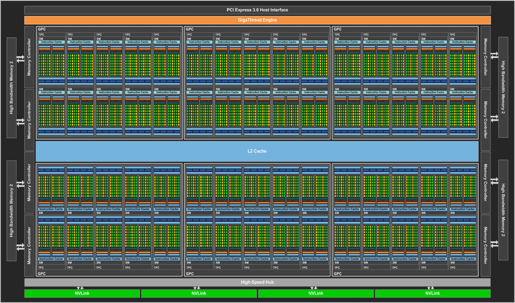
Memory Hierarchy

Custom Hardware for Matrix Multiply

Course Grained Parallelism (Asynchronous SGD)

On a worker, in each iteration

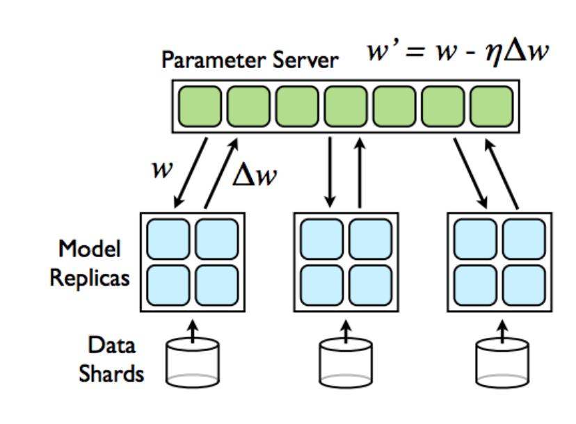• Fetch up-to-date parameters (weights) from parameter server
• Compute gradients with respect to these parameters
• Send gradients back to parameter server which upates the model

Synchronous SGD

• Each work waits for all other works to finish before getting updated weights from parameter server.
• Use "backup" workers to compensate for slow nodes.

PyTorch Distributed SGD

Workers share gradients to compute average gradient (allreduce). Each worker's solver then performs (what is assumed to be) an identical update operation.

Example

Setup TCGA example..

import numpy as np
import sklearn
from sklearn.model_selection import KFold

data = np.genfromtxt('bcsmall.csv',delimiter=',',skip_header=True)
X = data[:,2:]
Y = data[:,1]

X,Y

(array([[0., 0., 0., ..., 0., 0., 0.],
        [0., 0., 0., ..., 0., 0., 0.],
        [0., 0., 0., ..., 0., 0., 0.],
        ...,
        [0., 0., 0., ..., 0., 0., 0.],
        [0., 0., 0., ..., 0., 0., 0.],
        [0., 0., 0., ..., 0., 0., 0.]]),
 array([1., 1., 1., 1., 1., 1., 1., 1., 0., 1., 1., 1., 1., 1., 0., 1., 1.,
        1., 1., 0., 1., 1., 1., 1., 0., 1., 1., 1., 1., 0., 1., 1., 1., 1.,
        1., 1., 1., 1., 1., 1., 1., 1., 1., 1., 1., 1., 1., 1., 1., 1., 1.,
        1., 1., 0., 0., 1., 1., 1., 1., 0., 1., 1., 1., 1., 1., 1., 1., 1.,
        1., 1., 1., 1., 1., 1., 1., 1., 0., 1., 1., 1., 1., 1., 1., 1., 1.,
        1., 1., 1., 1., 1., 1., 1., 1., 1., 1., 1., 1., 1., 1., 1., 1., 1.,
        1., 1., 1., 1., 1., 1., 1., 1., 1., 1., 1., 1., 1., 0., 0., 1., 1.,
        1., 1., 1., 1., 1., 1., 1., 1., 1., 1., 1., 1., 1., 1., 1., 1., 1.,
        1., 1., 1., 1., 1., 1., 1., 1., 1., 1., 1., 1., 1., 0., 0., 1., 1.,
        1., 1., 1., 1., 1., 1., 1., 1., 1., 1., 1., 1., 1., 1., 1., 1., 1.,
        1., 1., 1., 1., 1., 1., 1., 1., 1., 1., 1., 1., 0., 1., 1., 1., 1.,
        1., 1., 1., 1., 1., 1., 1., 1., 1., 1., 1., 1., 1., 1., 1., 1., 1.,
        1., 1., 1., 1., 1., 1., 1., 1., 1., 1., 1., 1., 1., 1., 1., 1., 1.,
        1., 1., 1., 1., 1., 1., 1., 1., 1., 1., 1., 1., 1., 1., 1., 1., 0.,
        1., 1., 1., 0., 1., 1., 1., 1., 1., 1., 1., 1., 1., 1., 1., 1., 1.,
        1., 1., 1., 1., 1., 1., 1., 1., 1., 1., 1., 1., 1., 1., 1., 1., 1.,
        1., 1., 1., 1., 1., 1., 1., 1., 0., 1., 1., 1., 1., 1., 0., 1., 1.,
        0., 1., 1., 1., 1., 1., 1., 1., 1., 1., 1., 0., 1., 0., 1., 1., 1.,
        1., 1., 1., 1., 1., 1., 1., 1., 1., 1., 1., 1., 1., 1., 1., 1., 1.,
        1., 1., 1., 1., 1., 0., 1., 1., 0., 0., 0., 1., 0., 0., 0., 0., 0.,
        1., 0., 1., 0., 1., 1., 1., 1., 1., 1., 1., 1., 1., 0., 0., 1., 1.,
        1., 0., 1., 0., 0., 0., 0., 1., 0., 1., 0., 0., 0., 1., 1., 1., 1.,
        1., 1., 1., 1., 1., 1., 1., 1., 1., 1., 1., 1., 1., 1., 1., 1., 1.,
        1., 1., 1., 1., 1., 1., 1., 1., 1., 1., 1., 1., 1., 1., 1., 1., 1.,
        1., 1., 1., 1., 1., 1., 1., 1., 1., 1., 1., 1., 1., 1., 1., 1., 1.,
        1., 1., 1., 1., 0., 1., 1., 1., 1., 1., 1., 1., 1., 1., 1., 1., 1.,
        1., 1., 1., 1., 1., 1., 1., 1., 1., 1., 1., 1., 1., 1., 1., 1., 1.,
        1., 1., 1., 1., 1., 1., 0., 0., 0., 0., 0., 0., 0., 0., 0., 0., 0.,
        0., 0., 0., 0., 0., 0., 0., 0., 0., 0., 0., 0., 0., 0., 0., 0., 0.,
        0., 0., 0., 0., 0., 0., 0., 0., 1., 1., 0., 0., 0., 1., 1., 1., 1.,
        1., 1., 1., 1., 1., 1., 1., 1., 1., 1., 1., 1., 1., 1., 1., 1., 1.,
        1., 1., 1., 1., 1., 1., 1., 1., 1., 1., 1., 1., 1., 1., 1., 1., 1.,
        1., 1., 1., 1., 1., 1., 1., 1., 1., 1., 1., 1., 1., 1., 1., 1., 1.,
        1., 1., 1., 1., 1., 1., 1., 1., 1., 1., 1., 1., 1., 1., 1., 1., 1.,
        1., 1., 1., 1., 1., 1., 1., 1., 1., 1., 1., 1., 1., 1., 1., 1., 1.,
        1., 1., 1., 1., 1., 1., 1., 1., 1., 1., 1., 1., 1., 1., 1., 1., 1.,
        1., 1., 1., 1., 1., 1., 1., 1., 1., 1., 1., 1., 1., 1., 1., 1., 1.,
        1., 1., 1., 1., 1., 1., 1., 1., 1., 1., 1., 1., 1., 1., 1., 1., 1.,
        1., 1., 1., 1., 1., 1., 1., 1., 1., 1., 1., 1., 1., 1., 1., 1., 1.,
        1., 1., 1., 1., 1., 1., 1., 1., 1., 1., 1., 1., 1., 1., 1., 1., 1.,
        1., 1., 1., 1., 1., 1., 1., 1., 1., 0., 1., 1., 1., 1., 1., 1., 1.,
        1., 1., 1., 1., 1., 1., 1., 1., 1., 1., 1., 1., 1., 1., 1., 1., 1.,
        1., 1., 1., 1., 1., 1., 1., 1., 1., 1., 1., 1., 1., 1., 1., 1., 1.,
        1., 1., 1., 1., 1., 1., 1., 1., 1., 1., 1., 1., 1., 1., 1., 1., 1.,
        1., 1., 1., 1., 1., 1., 0., 1., 1., 1., 1., 1., 1., 1.]))

np.unique(X)

array([0., 1.])

kf = KFold(n_splits=3,shuffle=True)
(train, test) = list(kf.split(data))[0]
Xtrain = X[train]
Ytrain = Y[train]
Xtest = X[test]
Ytest = Y[test]

from sklearn.neural_network import MLPClassifier
mlp = MLPClassifier()
mlp.fit(Xtrain,Ytrain)

/home/dkoes/.local/lib/python3.10/site-packages/sklearn/neural_network/_multilayer_perceptron.py:691: ConvergenceWarning: Stochastic Optimizer: Maximum iterations (200) reached and the optimization hasn't converged yet.
  warnings.warn(

MLPClassifier()

In a Jupyter environment, please rerun this cell to show the HTML representation or trust the notebook.
On GitHub, the HTML representation is unable to render, please try loading this page with nbviewer.org.

mlp.get_params()

{'activation': 'relu',
 'alpha': 0.0001,
 'batch_size': 'auto',
 'beta_1': 0.9,
 'beta_2': 0.999,
 'early_stopping': False,
 'epsilon': 1e-08,
 'hidden_layer_sizes': (100,),
 'learning_rate': 'constant',
 'learning_rate_init': 0.001,
 'max_fun': 15000,
 'max_iter': 200,
 'momentum': 0.9,
 'n_iter_no_change': 10,
 'nesterovs_momentum': True,
 'power_t': 0.5,
 'random_state': None,
 'shuffle': True,
 'solver': 'adam',
 'tol': 0.0001,
 'validation_fraction': 0.1,
 'verbose': False,
 'warm_start': False}

plt.plot(mlp.loss_curve_);

from sklearn import metrics

print("Test on Train AUC",metrics.roc_auc_score(Ytrain,mlp.predict_proba(Xtrain)[:,1]))
print("Held out Test AUC",metrics.roc_auc_score(Ytest,mlp.predict_proba(Xtest)[:,1]))

Test on Train AUC 0.9999416501342047
Held out Test AUC 0.5201485461441213

Example 2

Cheminformatics data...

import numpy as np
import sklearn
from sklearn.model_selection import KFold

data = np.genfromtxt('compounds.fp',comments=None)
X = data[:,2:]
Y = data[:,1]

kf = KFold(n_splits=3,shuffle=True)
(train, test) = list(kf.split(data))[0]
Xtrain = X[train]
Ytrain = Y[train]
Xtest = X[test]
Ytest = Y[test]

mlp = MLPClassifier()
mlp.fit(Xtrain,Ytrain)

MLPClassifier()

In a Jupyter environment, please rerun this cell to show the HTML representation or trust the notebook.
On GitHub, the HTML representation is unable to render, please try loading this page with nbviewer.org.

plt.plot(mlp.loss_curve_);

print("Test on Train AUC",metrics.roc_auc_score(Ytrain,mlp.predict_proba(Xtrain)[:,1]))
print("Held out Test AUC",metrics.roc_auc_score(Ytest,mlp.predict_proba(Xtest)[:,1]))

Test on Train AUC 1.0
Held out Test AUC 0.9644503696319758

Effect of learning rate

for lr in [0.0001,0.001,0.01,0.1]:
    mlp = MLPClassifier(learning_rate_init=lr,max_iter=200)
    mlp.fit(Xtrain,Ytrain)
    plt.plot(mlp.loss_curve_)
plt.xlabel('Iteration'); plt.ylabel('Loss');

%%html
<div id="lrcolor" style="width: 500px"></div>
<script>

    var divid = '#lrcolor';
	jQuery(divid).asker({
	    id: divid,
	    question: "Which color is from the smallest learning rate?",
		answers: ["blue","orange","red","green"],
        server: "https://bits.csb.pitt.edu/asker.js/example/asker.cgi",
		charter: chartmaker})
    
$(".jp-InputArea .o:contains(html)").closest('.jp-InputArea').hide();


</script>

%%html
<div id="lrcolor2" style="width: 500px"></div>
<script>

    var divid = '#lrcolor2';
	jQuery(divid).asker({
	    id: divid,
	    question: "Which color is from the largest learning rate?",
		answers: ["blue","orange","red","green"],
        server: "https://bits.csb.pitt.edu/asker.js/example/asker.cgi",
		charter: chartmaker})
    
$(".jp-InputArea .o:contains(html)").closest('.jp-InputArea').hide();


</script>

for lr in [0.0001,0.001,0.01,0.1]:
    plt.plot([0,1],np.log10([lr,lr]),label=f'{lr}')
plt.legend();

You probably should not use sklearn to train neural nets for large datasets. There are several frameworks for fast (GPU optimized) neural net training.

• Torch http://torch.ch
• JAX https://github.com/google/jax
• TensorFlow https://www.tensorflow.org
• Keras https://keras.io/
• Caffe http://caffe.berkeleyvision.org
• Theano http://deeplearning.net/software/theano/

Let's Play!

http://playground.tensorflow.org/

Next time: deep learning and convolutional neural networks.