Generative Models

2/29/2024

print view

%%html
<script src="https://bits.csb.pitt.edu/preamble.js"></script>

Review

CNN

• Receptive field size of kernel; successive applications expand field incrementally
• Good for identifying spatial, local features and learning hierarchy of features

RNN

• Receptive field is what it has seen so far
  • But has trouble "remembering" what it has seen
  • LSTM is better at remembering

Attention

• Receptive field is entire input
• Needs positional encoding to be position-specific (spatially aware)

Generative vs. Discriminative

A generative model produces as output the input of a discriminative model: $P(X|Y=y)$ or $P(X,Y)$

$y \rightarrow$

Model

$ \rightarrow X$

Model

$ \rightarrow X,y$

Autoencoders

A neural network trained to generate its input.

https://en.wikipedia.org/wiki/Autoencoder

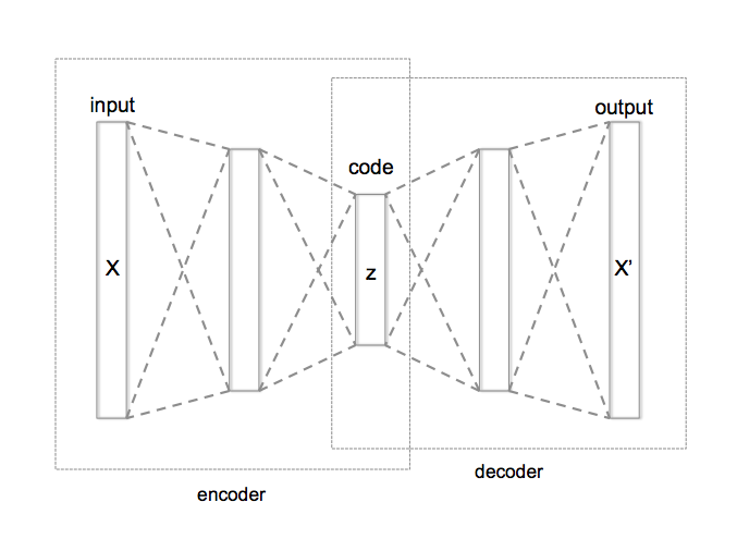
Autoencoders

Let's train an autoencoder on MNIST (input is 28x28).

import torch
import torch.nn as nn
import torch.nn.functional as F
from torchvision import datasets
from torchvision import transforms
train_data = datasets.MNIST(root='../data', train=True,transform=transforms.ToTensor())
test_data = datasets.MNIST(root='../data', train=False,transform=transforms.ToTensor())
train_loader = torch.utils.data.DataLoader(train_data,batch_size=100,shuffle=True)
test_loader = torch.utils.data.DataLoader(test_data,batch_size=100,shuffle=False)

class MyAutoEncoder(nn.Module):
    def __init__(self, latent_size):  #initialize submodules here - this defines our network architecture
        super(MyAutoEncoder, self).__init__()
        self.conv1 = nn.Conv2d(in_channels=1, out_channels=64, \
                               kernel_size=7, stride=1, padding=X) 
        self.conv2 = nn.Conv2d(in_channels=64, out_channels=64, \
                               kernel_size=7, stride=1, padding=X)
        self.latent_size = latent_size
        self.fc_encode = nn.Linear(3136, latent_size) 
        self.fc_decode1 = nn.Linear(latent_size, 500)
        self.fc_decode2 = nn.Linear(500, 784)
        

    def forward(self, x): # this actually applies the operations
        inshape = x.shape
        x = self.conv1(x)
        x = F.relu(x)
        x = F.max_pool2d(x, kernel_size=2, stride=2)  # POOL    
        x = self.conv2(x)
        x = F.relu(x)
        x = F.max_pool2d(x, kernel_size=2, stride=2) # POOL
        x = torch.flatten(x, 1)
        x = latent = self.fc_encode(x)
        x = F.softplus(self.fc_decode1(x))  #softplus is smooth approx of relu
        x = F.softplus(self.fc_decode2(x))
        return x.reshape(inshape), latent #return latent space representation
    
    def generate(self,x):
        with torch.no_grad():
            batchsize = x.shape[0]
            x = F.softplus(self.fc_decode1(x))  #softplus is smooth approx of relu
            x = F.softplus(self.fc_decode2(x))
            return x.reshape((batchsize,1,28,28))

%%html
<div id="whatpad" style="width: 500px"></div>
<script>

    var divid = '#whatpad';
	jQuery(divid).asker({
	    id: divid,
	    question: "What is X?",
		answers: ["0","1","2","3","7"],
        server: "https://bits.csb.pitt.edu/asker.js/example/asker.cgi",
		charter: chartmaker})
    
$(".jp-InputArea .o:contains(html)").closest('.jp-InputArea').hide();

</script>

def train_ae(latent_size):
    model = MyAutoEncoder(latent_size).to('cuda')
    optimizer = torch.optim.Adam(model.parameters()) # need to tell optimizer what it is optimizing
    losses = []
    for epoch in range(10):
        for i, (img,label) in enumerate(train_loader):
            optimizer.zero_grad()  # IMPORTANT!
            img = img.to('cuda') #don't care about label!
            output, latent = model(img)
            loss = F.mse_loss(output,img)
            loss.backward()
            optimizer.step()
            losses.append(loss.item())
            if i % 1000 == 0:
                print("epoch %d, iteration %d, loss %f"%(epoch,i,loss.item()))
    return model,losses

%%time
model100, losses100 = train_ae(100)

epoch 0, iteration 0, loss 0.466085
epoch 1, iteration 0, loss 0.012018
epoch 2, iteration 0, loss 0.008846
epoch 3, iteration 0, loss 0.007461
epoch 4, iteration 0, loss 0.006674
epoch 5, iteration 0, loss 0.005437
epoch 6, iteration 0, loss 0.005378
epoch 7, iteration 0, loss 0.004438
epoch 8, iteration 0, loss 0.004234
epoch 9, iteration 0, loss 0.003591
CPU times: user 1min 9s, sys: 561 ms, total: 1min 10s
Wall time: 1min 9s

import matplotlib.pyplot as plt
%matplotlib inline
plt.plot(losses100)
plt.ylim(0,.2);

from matplotlib import cm

def plot_imgs(model):
    batch = next(iter(test_loader))
    imgs = batch[0]
    labels = batch[1]
    genbatch, latent = model(imgs.to('cuda'))
    genbatch = genbatch.detach().cpu().numpy() # remove from computation graph and move to CPU
    fig,axes=plt.subplots(10,2,figsize=(4,20))
    for i in range(10):    
        axes[i][0].imshow(genbatch[i][0],cmap=cm.Greys_r)
        axes[i][1].imshow(imgs[i][0],cmap=cm.Greys_r)    
    axes[0][0].set_title('Generated')
    axes[0][1].set_title('True');
    return latent, labels

latent100, _ = plot_imgs(model100)

Latent Vector

latent100[0]

tensor([ 1.1821e+00,  2.7541e-01,  5.2303e-01,  5.2842e-01,  7.2577e-01,
        -2.9952e+00, -2.8875e-01,  2.2576e-01, -2.9301e+00,  2.4102e-01,
        -6.8178e+00, -2.5452e+00, -1.4065e+00, -4.5583e+00, -3.0011e+00,
        -2.2526e+00,  1.2774e-01,  1.1715e+00,  3.4959e+00, -8.9686e-02,
        -3.1287e-03,  7.3937e-01, -1.8150e+00, -2.5783e+00, -2.5707e+00,
         2.7477e+00,  5.1790e+00,  2.7054e+00, -7.5436e-01,  2.3868e+00,
        -2.4104e+00,  6.0113e+00, -7.5003e-01, -4.1176e+00,  4.0544e+00,
         3.4794e+00,  1.5832e+00,  9.4781e-01, -1.4915e+00, -1.5748e+00,
        -2.6026e+00, -1.6287e+00,  1.5664e-01,  1.3643e+00, -2.0033e+00,
        -6.9889e+00,  1.3188e-01,  1.0948e-01, -2.0367e+00,  6.9195e-01,
         2.3225e+00, -4.8781e+00,  3.3334e+00, -2.7200e+00, -2.5480e+00,
         6.8248e-01,  3.1682e+00,  2.1084e+00, -3.4232e+00,  1.3786e+00,
        -1.7187e+00, -1.0005e+00, -5.6148e-01,  1.5399e+00,  1.2128e+00,
         2.1750e-01,  1.3939e+00, -1.1122e+00, -7.8315e-02,  3.1608e+00,
        -5.9425e-02,  1.4927e+00, -2.2714e+00,  4.2443e+00, -1.6202e+00,
        -7.5918e-02,  6.6270e-02, -4.6522e-01,  1.5404e+00, -4.8643e-02,
        -4.1407e+00,  8.8498e-01, -1.0276e+00, -5.4198e+00,  1.6866e+00,
        -1.7033e+00, -1.4342e+00,  1.0432e+00,  1.3793e+00, -2.4997e+00,
         3.0524e-01,  4.1902e-01, -2.5756e-01, -8.7851e-01, -4.5882e-01,
         6.1373e-01, -2.8110e+00,  9.3498e-01, -1.2536e+00,  1.4744e+00],
       device='cuda:0', grad_fn=<SelectBackward0>)

%%html
<div id="redlat" style="width: 500px"></div>
<script>

    var divid = '#redlat';
	jQuery(divid).asker({
	    id: divid,
	    question: "What do you expect to happen if we reduce the size of the latent vector?",
		answers: ["Smaller error","Similar error","Larger error"],
        server: "https://bits.csb.pitt.edu/asker.js/example/asker.cgi",
		charter: chartmaker})
    
$(".jp-InputArea .o:contains(html)").closest('.jp-InputArea').hide();

</script>

%%time
model10, losses10 = train_ae(10)

epoch 0, iteration 0, loss 0.461887
epoch 1, iteration 0, loss 0.022974
epoch 2, iteration 0, loss 0.017564
epoch 3, iteration 0, loss 0.018944
epoch 4, iteration 0, loss 0.018463
epoch 5, iteration 0, loss 0.017074
epoch 6, iteration 0, loss 0.015522
epoch 7, iteration 0, loss 0.016885
epoch 8, iteration 0, loss 0.015761
epoch 9, iteration 0, loss 0.016013
CPU times: user 1min 9s, sys: 182 ms, total: 1min 9s
Wall time: 1min 7s

model2, losses2 = train_ae(2)

epoch 0, iteration 0, loss 0.493047
epoch 1, iteration 0, loss 0.050635
epoch 2, iteration 0, loss 0.047277
epoch 3, iteration 0, loss 0.048770
epoch 4, iteration 0, loss 0.050351
epoch 5, iteration 0, loss 0.048944
epoch 6, iteration 0, loss 0.049963
epoch 7, iteration 0, loss 0.048087
epoch 8, iteration 0, loss 0.050051
epoch 9, iteration 0, loss 0.046337

plt.plot(losses100,label='100')
plt.plot(losses10,label='10')
plt.plot(losses2,label='2')

plt.ylim(0,.2)
plt.legend();

latent,_ = plot_imgs(model10)

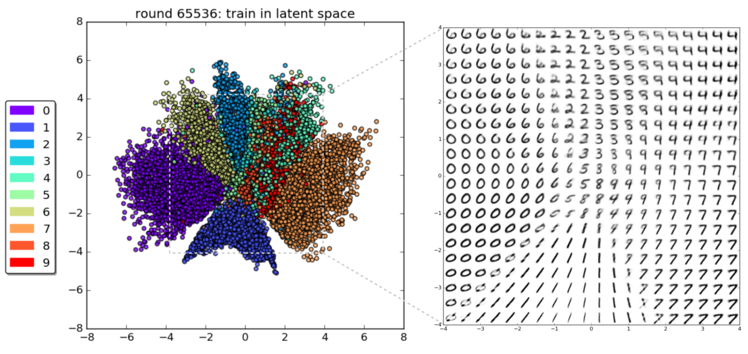
latent, labels = plot_imgs(model2)

import seaborn as sns
latent = latent.detach().cpu().numpy()
sns.scatterplot(x=latent[:,0],y=latent[:,1],hue=labels,palette='bright');

An autoencoder is dimensionality reduction technique

Latent Space

http://blog.fastforwardlabs.com/2016/08/12/introducing-variational-autoencoders-in-prose-and.html

Latent Space Arithmetic

https://arxiv.org/pdf/1707.05776.pdf

Latent Spaces for Molecules

https://arxiv.org/abs/1610.02415

1% - 70% of output valid SMILES

Our Latent Space

import numpy as np
l = latent100.detach().cpu().numpy()
diff = l[10]-l[0]
N = 10
L = torch.Tensor(np.array([l[0]+frac*diff for frac in np.linspace(0,1,N)]))
pi = model100.generate(L.to('cuda')).detach().cpu().numpy()

plt.figure(figsize=(16,4))
for i in range(N):
    plt.subplot(1,N,i+1)
    plt.imshow(pi[i].reshape((28,28)),cmap=cm.Greys_r)

Generating from Scratch

newL = torch.Tensor(np.random.normal(size=(5,100)))
pgen = model100.generate(newL.to('cuda')).cpu().numpy()

plt.figure(figsize=(10,4))
for i in range(5):
    plt.subplot(1,5,i+1)
    plt.imshow(pgen[i].reshape((28,28)),cmap=cm.Greys_r)

Variational Autoencoder

An autoencoder is good for constructing a compressed representation of the input. For generating new inputs, we want to impose some constraints on the latent space to make it more amenable to sampling.

http://kvfrans.com/variational-autoencoders-explained/

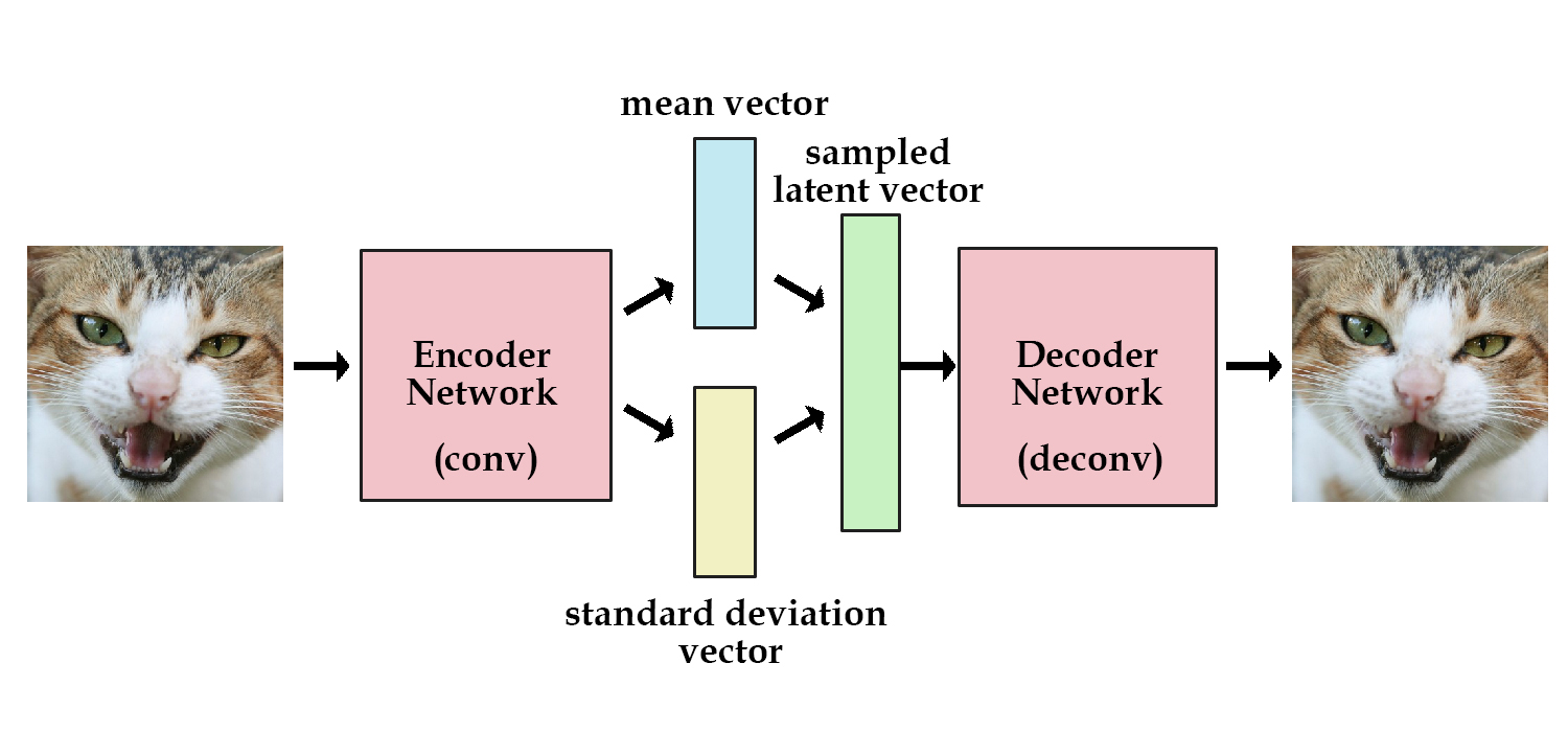
Reparameterization Trick

Problem: Sampling from a distribution is not differentiable.

Solution: Sample from $\mathcal{N}(0,1)$ (not differentiable) and scale (differentiable) by a predicted mean and standard deviation.

$$ \epsilon = \mathcal{N}(0,1) $$ $$ z = \mu + \sigma \cdot \epsilon$$

$z$ is now a sample from $\mathcal{N}(\mu,\sigma)$

Variational Autoencoder

Instead of generating the latent vector directly, we generate probability distributions from which the latent vector is sampled. To regularize this distributions we introduce a Kullback–Leibler divergence loss.

Kullback-Leibler divergence, $D_{KL}$ is a measure of how different two probability distributions are.

"A simple interpretation of the divergence of P from Q is the expected excess surprise from using Q as a model when the actual distribution is P."

%%html
<div id="klsame" style="width: 500px"></div>
<script>

    var divid = '#klsame';
	jQuery(divid).asker({
	    id: divid,
	    question: "Does KL(P||Q) == KL(Q||P)?",
		answers: ["Yes","No"],
        server: "https://bits.csb.pitt.edu/asker.js/example/asker.cgi",
		charter: chartmaker})
    
$(".jp-InputArea .o:contains(html)").closest('.jp-InputArea').hide();


</script>

Kullback-Leibler Divergence

"Usually, $P$ represents the data, the observations, or a measured probability distribution. Distribution $Q$ represents instead a theory, a model, a description or an approximation of $P$. The Kullback–Leibler divergence is then interpreted as the average difference of the number of bits required for encoding samples of $P$ using a code optimized for $Q$ rather than one optimized for $P$."

$$D_{\mathrm{KL}}\left( P || Q\right) = \int p(x)\log\left(\frac{p(x)}{q(x)}\right) dx = \mathbb{E}_p[ \log p(x) - \log q(x) ]$$

We will condition our generated distributions to be similar to a standard normal distribution.

Derivation

%%html
<div id="whatisk" style="width: 500px"></div>
<script>
$('head').append('<link rel="stylesheet" href="https://bits.csb.pitt.edu/asker.js/themes/asker.default.css" />');

    var divid = '#whatisk';
	jQuery(divid).asker({
	    id: divid,
	    question: "What is k?",
		answers: ["latent vector length","batch size","infinity","pixels"],
        server: "https://bits.csb.pitt.edu/asker.js/example/asker.cgi",
		charter: chartmaker})
    
$(".jp-InputArea .o:contains(html)").closest('.jp-InputArea').hide();


</script>

Variational Autoencoder

Let's make our autoencoder variational...

class MyVAE(nn.Module):
    def __init__(self, latent_size):  #initialize submodules here - this defines our network architecture
        super(MyVAE, self).__init__()
        self.conv1 = nn.Conv2d(in_channels=1, out_channels=64, kernel_size=7, stride=1, padding=X) 
        self.conv2 = nn.Conv2d(in_channels=64, out_channels=64, kernel_size=7, stride=1, padding=X)
        self.latent_size = latent_size
        self.fc_encode_mean = nn.Linear(3136, latent_size) 
        self.fc_encode_log_sigma_sq = nn.Linear(3136, latent_size) 

        self.fc_decode1 = nn.Linear(latent_size, 500)
        self.fc_decode2 = nn.Linear(500, 784)
        

    def forward(self, x): # this actually applies the operations
        inshape = x.shape
        x = self.conv1(x)
        x = F.relu(x)
        x = F.max_pool2d(x, kernel_size=2, stride=2)  # POOL    
        x = self.conv2(x)
        x = F.relu(x)
        x = F.max_pool2d(x, kernel_size=2, stride=2) # POOL
        x = torch.flatten(x, 1)
        
        #two latent vectors
        mean = self.fc_encode_mean(x)
        log_sigma_sq = self.fc_encode_log_sigma_sq(x)
        
        #sample according to mean/sigma
        std = torch.exp(0.5*log_sigma_sq)
        eps = torch.randn_like(std)
        z = eps*std+mean
        
        x = F.softplus(self.fc_decode1(z))  #softplus is smooth approx of relu
        x = F.softplus(self.fc_decode2(x))
        return x.reshape(inshape), (mean, log_sigma_sq, z) #return latent space representation
    
    def generate(self,batchsize,std=1):
        with torch.no_grad():
            x = torch.normal(0, std,size=(batchsize,self.latent_size)).to('cuda')
            x = F.softplus(self.fc_decode1(x))  #softplus is smooth approx of relu
            x = F.softplus(self.fc_decode2(x))
            return x.reshape((batchsize,1,28,28))

def train_vae(latent_size,mult=1):
    model = MyVAE(latent_size).to('cuda')
    optimizer = torch.optim.Adam(model.parameters()) # need to tell optimizer what it is optimizing
    losses = []
    for epoch in range(10):
        for i, (img,label) in enumerate(train_loader):
            optimizer.zero_grad()  # IMPORTANT!
            img = img.to('cuda') #don't care about label!
            output, (mean, log_sigma_sq, z) = model(img)
            l2loss = mult*F.mse_loss(output,img)        
            klloss = -0.5*torch.mean(torch.sum(\
                            1+log_sigma_sq - torch.square(mean) - \
                                torch.exp(log_sigma_sq),dim=1),dim=0)
            loss = l2loss+klloss
            loss.backward()
            optimizer.step()
            losses.append(loss.item())
            if i % 1000 == 0:
                print("epoch %d, iteration %d, losses %f = %f + %f"%\
                      (epoch,i,loss.item(),l2loss.item(),klloss.item()))
    return model,losses

%%time
model100,losses100 = train_vae(100)

epoch 0, iteration 0, losses 0.778504 = 0.506249 + 0.272255
epoch 1, iteration 0, losses 0.065730 = 0.065730 + -0.000000
epoch 2, iteration 0, losses 0.067433 = 0.067433 + 0.000000
epoch 3, iteration 0, losses 0.066223 = 0.066223 + 0.000000
epoch 4, iteration 0, losses 0.066709 = 0.066709 + 0.000000
epoch 5, iteration 0, losses 0.067264 = 0.067264 + 0.000000
epoch 6, iteration 0, losses 0.071659 = 0.071659 + 0.000000
epoch 7, iteration 0, losses 0.068089 = 0.068088 + 0.000001
epoch 8, iteration 0, losses 0.065957 = 0.065956 + 0.000001
epoch 9, iteration 0, losses 0.068220 = 0.068219 + 0.000000
CPU times: user 1min 14s, sys: 259 ms, total: 1min 14s
Wall time: 1min 12s

genimgs = model100.generate(10).cpu().numpy()
fig, axes = plt.subplots(1,10,figsize=(16,4))
for i in range(10):
    axes[i].imshow(genimgs[i][0],cmap=cm.Greys_r)

latent, labels = plot_imgs(model100);

plt.hist(latent[2].detach().cpu().numpy().flatten(),bins=100,label='z');

Posterior Collapse!

The posterior (our desired distribution) has "collapsed" onto the prior distribution we are fitting with the KL divergence loss.

How to fix?

%%time
model100,losses100 = train_vae(100,1000)

epoch 0, iteration 0, losses 489.381409 = 489.018707 + 0.362690
epoch 1, iteration 0, losses 55.710548 = 49.215897 + 6.494653
epoch 2, iteration 0, losses 50.112415 = 40.437679 + 9.674735
epoch 3, iteration 0, losses 46.108665 = 36.279514 + 9.829151
epoch 4, iteration 0, losses 43.777828 = 34.007973 + 9.769855
epoch 5, iteration 0, losses 40.536324 = 29.290428 + 11.245897
epoch 6, iteration 0, losses 39.444569 = 28.167974 + 11.276593
epoch 7, iteration 0, losses 42.040955 = 30.187609 + 11.853347
epoch 8, iteration 0, losses 41.522102 = 29.518663 + 12.003438
epoch 9, iteration 0, losses 42.298878 = 29.080904 + 13.217975
CPU times: user 1min 15s, sys: 210 ms, total: 1min 15s
Wall time: 1min 12s

latent, labels = plot_imgs(model100);

genimgs = model100.generate(10).cpu().numpy()
fig, axes = plt.subplots(1,10,figsize=(16,4))
for i in range(10):
    axes[i].imshow(genimgs[i][0],cmap=cm.Greys_r)

plt.hist(latent[2].detach().cpu().numpy().flatten(),bins=100,label='z');

Generative Models of the Cell

https://arxiv.org/pdf/1705.00092.pdf

https://drive.google.com/file/d/0B2tsfjLgpFVhMnhwUVVuQnJxZTg/view

Generative Adversarial Networks

https://arxiv.org/abs/1406.2661 https://youtu.be/G06dEcZ-QTg

Training a GAN

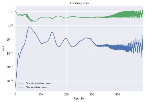
The loss is not necessarily a good indicator and for now, the most reliable way to check if their output makes sense is to put the output in front of an actual person. http://www.rricard.me/machine/learning/generative/adversarial/networks/keras/tensorflow/2017/04/05/gans-part2.html

https://towardsdatascience.com/gan-ways-to-improve-gan-performance-acf37f9f59b

An abbreviated GAN Tour

https://machinelearningmastery.com/tour-of-generative-adversarial-network-models/

We often want to condition our generated inputs in some way.

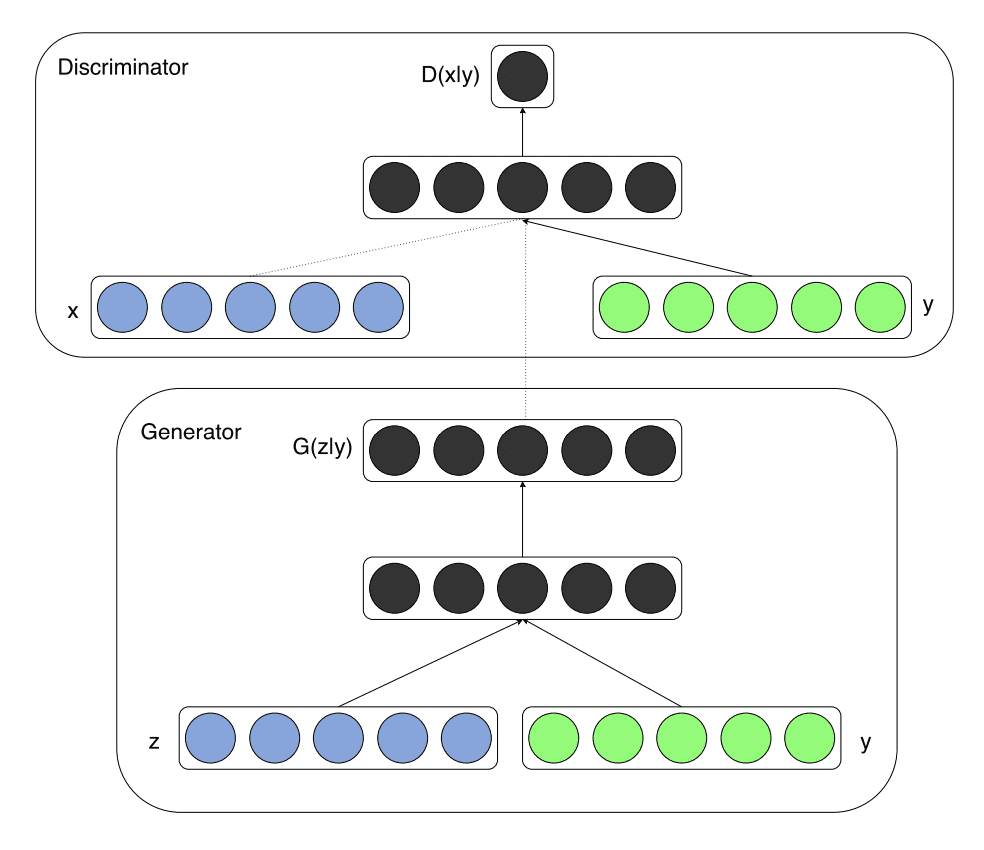
Conditional GAN

Both the discriminator and generator are conditioned on some variable (e.g., for MNIST we might condition on the label).

https://arxiv.org/abs/1411.1784

pix2pix

Can condition on an entire image. https://phillipi.github.io/pix2pix/

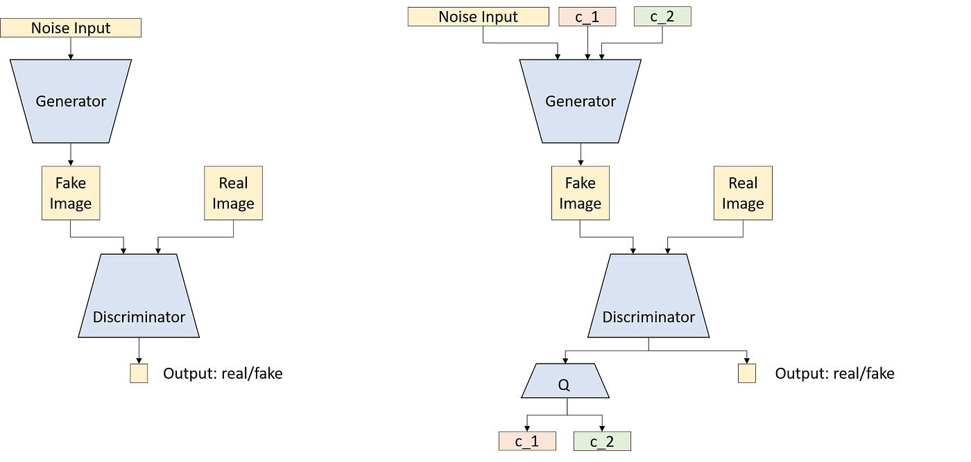
InfoGAN

You do not need to know what the labels are, only that there are labels (or other conditional properties). A network Q is expected to predict the conditional variable (label) used to generate the image from the image.

https://arxiv.org/abs/1606.03657

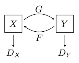
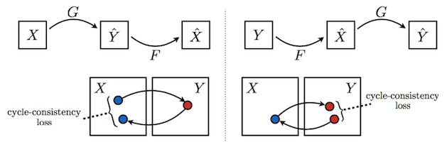
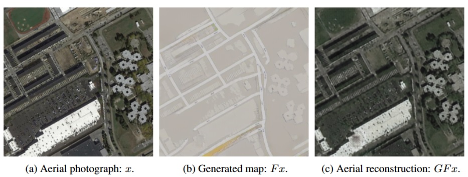
CycleGAN

Unlike pix2pix, you do not need matched pairs to convert between image domains.

https://medium.com/coding-blocks/introduction-to-cyclegans-1dbdb8fbe781

https://techcrunch.com/2018/12/31/this-clever-ai-hid-data-from-its-creators-to-cheat-at-its-appointed-task/

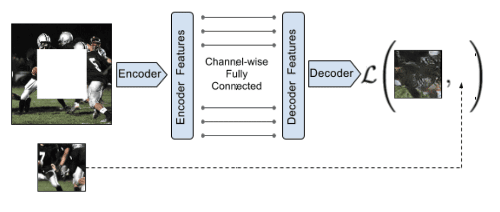
Context Encoders

The missing part of a picture is filled in. The doesn't have to use a GAN, but in practice an adversarial loss improves the result.

https://arxiv.org/abs/1604.07379

Molecular Context Encoders

https://pubs.rsc.org/en/content/articlehtml/2022/sc/d1sc05976a

And many more...

https://github.com/hindupuravinash/the-gan-zoo