%%html
<script src="https://bits.csb.pitt.edu/preamble.js"></script>
The RTX 4090 GPU has 16,384 cores and 128 streaming multiprocessors. A CUDA kernel is launched using 64 blocks and and 1024 threads:
Add<<<64, 1024>>>(A, B, C)
%%html
<div id="cudaq" style="width: 500px"></div>
<script>

    var divid = '#cudaq';
	jQuery(divid).asker({
	    id: divid,
	    question: "At a given moment, how many threads of this kernel can be executing concurrently?",
		answers: ["64","1024","8192","16384","65536"],
        server: "https://bits.csb.pitt.edu/asker.js/example/asker.cgi",
		charter: chartmaker})

$(".jp-InputArea .o:contains(html)").closest('.jp-InputArea').hide();


</script>
Recall
Backpropagation 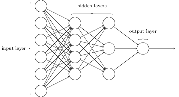
- Feedforward.
$$a^{l} = \sigma(z^{l})$$
2. Compute output error
$$\delta^{N} = \nabla_a L \odot \sigma'(z^N)$$
3. Backpropagate the error
$$\delta^{l} = ((w^{l+1})^T \delta^{l+1}) \odot
\sigma'(z^{l})$$
4. Calculate gradients
$$\frac{\partial L}{\partial w^l_{jk}} = a^{l-1}_k \delta^l_j \text{ and } \frac{\partial L}{\partial b^l_j} = \delta^l_j$$
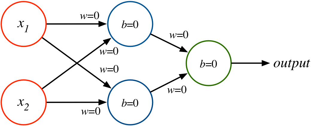
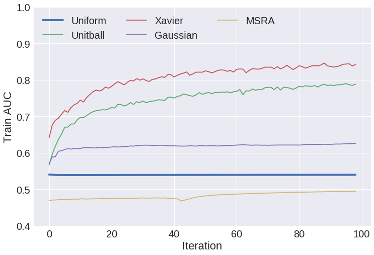
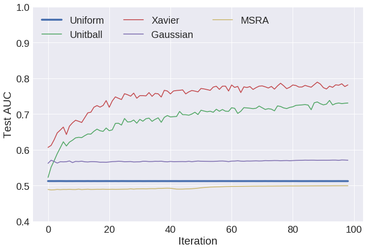
Weight Initialization
What happens with back propagation if weights/biases are initialized to zero with ReLU? Sigmoid?
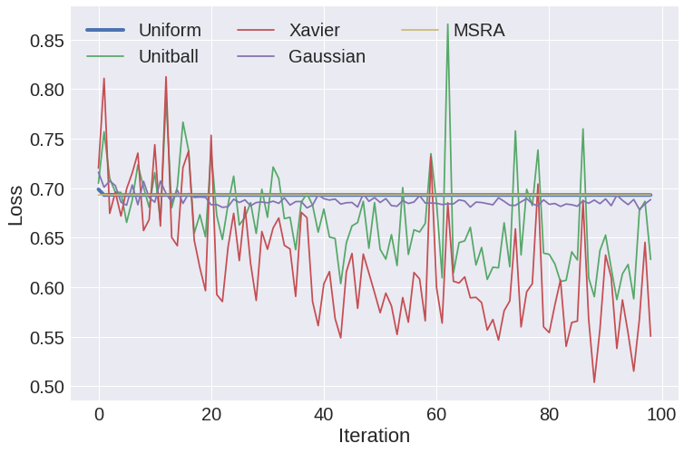
Weight Initialization
- constant - (e.g. all zero), almost never a good idea
- uniform - sample uniformly from range $(a,b)$, e.g. $(0,1)$
- positive unitball - sample from $(0,1)$ such that layer weights sum to 1
- Gaussian - sample from normal distribution
- Xavier - sample uniform distribution with range determined by fan-in/fan-out
- MSRA - sample normal distribution with variance determined by fan-in/fan-out
- https://arxiv.org/pdf/1502.01852.pdf
- compared to Xavier, works better with non-linear activation functions
Xavier Initialization
Sample from uniform distribution $(-a,a)$ where $$a = \sqrt{\frac{6}{\mathrm{fan}_\mathrm{in}+\mathrm{fan}_\mathrm{out}}}$$
The goal here is to maintain a constant variance both forwards and backwards.
Sometimes multiply by an activation function dependent scaling factor (gain).
Weight Initialization
Weight Initialization
Weight Initialization
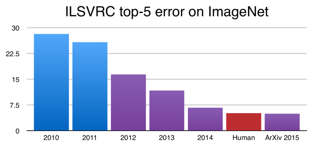
Deep Learning
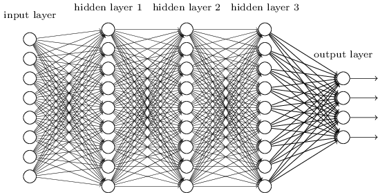
A deep network is not more powerful (recall can approximate any function with a single layer), but may be more concise - can approximate some functions with many fewer nodes.
%%html
<div id="deepq" style="width: 500px"></div>
<script>
    var divid = '#deepq';
	jQuery(divid).asker({
	    id: divid,
	    question: "Intuitively, which part of a deep network will learn faster?",
		answers: ["Early layers","Later layers","Uniform"],
        server: "https://bits.csb.pitt.edu/asker.js/example/asker.cgi",
		charter: chartmaker})

$(".jp-InputArea .o:contains(html)").closest('.jp-InputArea').hide();


</script>
Vanishing Gradients
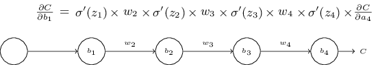
Since weights tend to start out small and sigmoid derivatives are small, gradients tend to be smaller earlier in the network, resulting in slower learning (smaller weight updates).
However, if weights are large, the opposite can happen - the exploding gradient problem.
The unstable gradient problem means that layers tend to learn at different speeds.
%%html
<div id="vangrad" style="width: 500px"></div>
<script>

    var divid = '#vangrad';
	jQuery(divid).asker({
	    id: divid,
	    question: "Intuitively, which activation function is less likely to result in vanishing gradients?",
		answers: ["Sigmoid","tanh","ReLU"],
        server: "https://bits.csb.pitt.edu/asker.js/example/asker.cgi",
		charter: chartmaker})

$(".jp-InputArea .o:contains(html)").closest('.jp-InputArea').hide();


</script>
ReLUs
ReLUs tend to result in faster training, but they can die.
LeakyReLU's are a proposed workaround.
Also, exponential linear units (ELUs) $$ y = \left\{ \begin{array}{lr} x & \mathrm{if} \; x > 0 \\ \alpha (e^x-1) & \mathrm{if} \; x \le 0 \end{array} \right. $$
plt.axhline(y=0, color='k')
plt.axvline(x=0, color='k')
plt.plot(x,np.maximum(0,x)+0.1*(np.exp(np.minimum(x,0))-1),linewidth=3,label="alpha = 0.1");
plt.plot(x,np.maximum(0,x)+(np.exp(np.minimum(x,0))-1),linewidth=1,label="alpha = 1.0");
plt.legend(loc='best');

Convolution Filters
A filter applies a convolution kernel to an image.
The kernel is represented by an $n$x$n$ matrix where the target pixel is in the center.
The output of the filter is the sum of the products of the matrix elements with the corresponding pixels.
Examples (from Wikipedia:
 |

|

|
| Identity | Blur | Edge Detection |
Edges
import numpy as np
import matplotlib.pyplot as plt
%matplotlib inline
from matplotlib import cm
from PIL import Image, ImageFilter
dog = Image.open('figs/dog.png')
f = plt.figure(figsize=(12,6))
f.add_subplot(1, 2, 1)
plt.imshow(np.array(dog),cmap = cm.Greys_r)
f.add_subplot(1, 2, 2)
plt.imshow(np.array(dog.filter(ImageFilter.FIND_EDGES)), cmap=cm.Greys_r)
print(ImageFilter.FIND_EDGES.filterargs)
((3, 3), 1, 0, (-1, -1, -1, -1, 8, -1, -1, -1, -1))

Edges
What would these convolutions do?
v = np.array([
        [-1,0,1],
        [-1,0,1],
        [-1,0,1]])

h = np.array([
        [-1,-1,-1],
        [0,0,0],
        [1,1,1]])
f = plt.figure(figsize=(12,6))
f.add_subplot(1, 2, 1)
plt.imshow(np.array(dog.filter(ImageFilter.Kernel((3,3),v.flatten(),1))), cmap=cm.Greys_r)
f.add_subplot(1, 2, 2)
plt.imshow(np.array(dog.filter(ImageFilter.Kernel((3,3),h.flatten(),1))), cmap=cm.Greys_r);

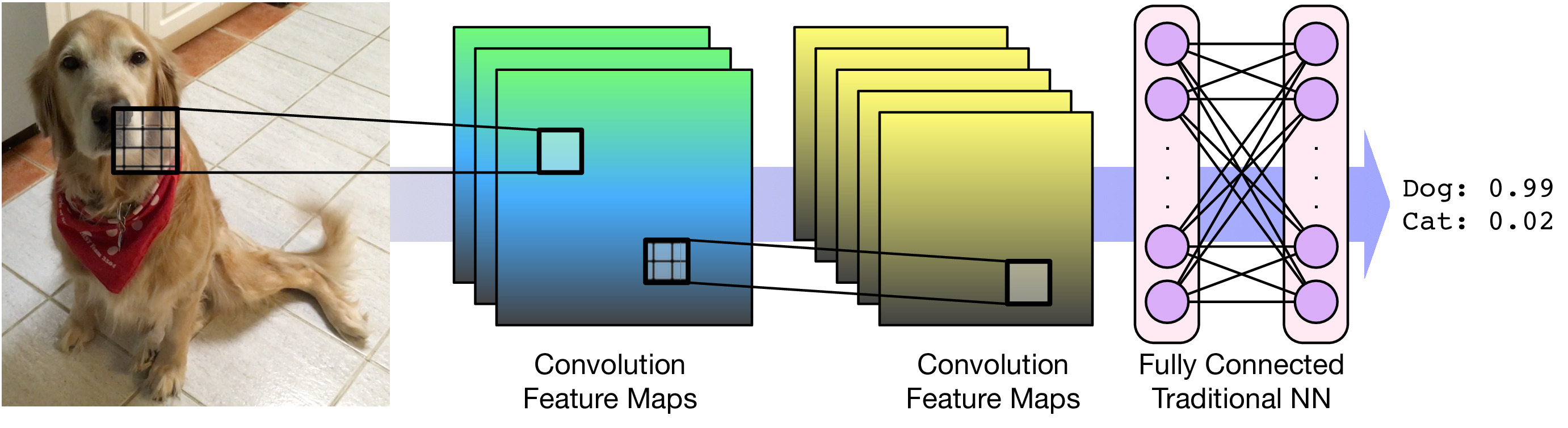
Feature Maps
We can think of a kernel as identifying a feature in an image and the resulting image as a feature map that has high values (white) where the feature is present and low values (black) elsewhere.
Feature maps retain the spatial relationship* between features present in the original image.*
Each feature map is called a channel. For color images, the input starts with 3 channels. Successive layers will have an output channel for each kernel.
Convolutional Layers
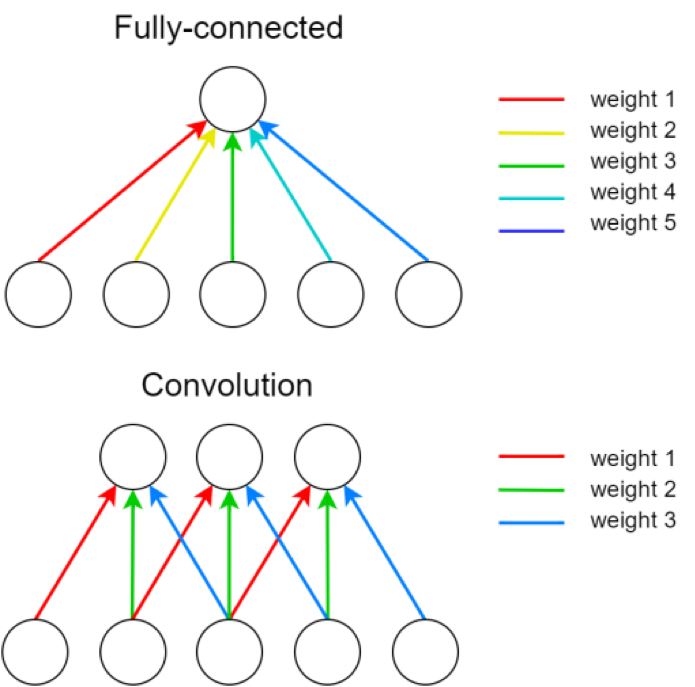 A single kernel is applied across the input. For each output feature map there is a single set of weights.
Convolutional Layers
For images, each pixel is an input feature. Each hidden layer is a set of feature maps.
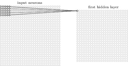
Consider an input image with 100 pixels. In a classic neural network, we hook these pixels up to a hidden layer with 10 nodes. In a CNN, we hook these pixels up to a convolutional layer with a 3x3 kernel and 10 output feature maps.
%%html
<div id="weightcnt" style="width: 500px"></div>
<script>
    var divid = '#weightcnt';
	jQuery(divid).asker({
	    id: divid,
	    question: "Which network has more parameters to learn?",
		answers: ["Classic","CNN"],
        server: "https://bits.csb.pitt.edu/asker.js/example/asker.cgi",
		charter: chartmaker})

$(".jp-InputArea .o:contains(html)").closest('.jp-InputArea').hide();


</script>
Convolution Parameters
- kernel_size size of kernel
- stride how much to shift kernel
- padding amount of implicit padding at edges (usually zero, but can extend/reflect/wrap values)
- dilation the spacing between the kernel points
- groups how inputs connect to outputs - default is all inputs (channels) effect all outputs. That is, your kernel has C x W x H weights.
https://github.com/vdumoulin/conv_arithmetic/blob/master/README.md
We apply a convolution with kernel_size 5, stride 3, and padding 0 to a 20x20 image
%%html
<div id="stridecnn" style="width: 500px"></div>
<script>
    var divid = '#stridecnn';
	jQuery(divid).asker({
	    id: divid,
	    question: "What will be the size of the output?",
		answers: ["6x6","5x5","20x20","17x17","7x7"],
        server: "https://bits.csb.pitt.edu/asker.js/example/asker.cgi",
		charter: chartmaker})

$(".jp-InputArea .o:contains(html)").closest('.jp-InputArea').hide();


</script>

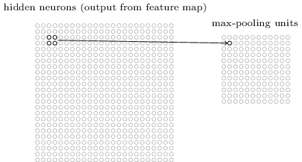
Pooling
Pooling layers apply a fixed convolution (usually the non-linear MAX kernel). The kernel is usually applied with a stride to reduce the size of the layer.
- faster to train
- fewer parameters to fit
- less sensitive to small changes (MAX)
Deep Learning Frameworks
Three different approaches to defining a network.
- Declarative Describe the network using some custom format.
- Programmatic Static Graph Creation Build the network using code.
- Programmatic Dynamic Graph Creation The network is built as you perform its constitutive operations
Declarative Example: Caffe
layer {
  name: "unit1_pool"
  type: "Pooling"
  bottom: "data"
  top: "unit1_pool"
  pooling_param {
    pool: AVE
    kernel_size: 2
    stride: 2
  }
}
layer {
  name: "unit1_conv"
  type: "Convolution"
  bottom: "unit1_pool"
  top: "unit1_conv"
  convolution_param {
    num_output: 32
    pad: 1
    kernel_size: 3
    stride: 1
    weight_filler {
      type: "xavier"
      symmetric_fraction: 1.0
    }
  }
}
Static Graph Example:  TensorFlow 1.0
TensorFlow is Google's open-source library for computation on dataflow graphs.
Data is represented as tensors, multi-dimensional blocks of data.
Each node in the dataflow graph is executed on a single resource (e.g. CPU or GPU).
Nodes are executed as data becomes available.
This is a very generic, low-level library.

Building the Graph
The first step of using TensorFlow is building the dataflow graph. This is done programmatically in Python.
Placeholders are inputs into the dataflow graph and must be declared as such.
Each function returns a graph node - it does not actually perform the operation.
Note: Placeholders are gone in Tensorflow 2.0, which follows an eager execution model (dynamic graph creation).
x = tf.placeholder(tf.float32, shape=[None, 28, 28, 1])
y_ = tf.placeholder(tf.float32, shape=[None, 10])

def weight_variable(shape):  #randomly sample weights
    initial = tf.truncated_normal(shape, stddev=0.1)
    return tf.Variable(initial)

def bias_variable(shape):  # start with positive offset for ReLUs
    initial = tf.constant(0.1, shape=shape)
    return tf.Variable(initial)

def conv2d(x, W):
    return tf.nn.conv2d(x, W, strides=[1, 1, 1, 1], padding='SAME')

def max_pool_2x2(x):
    return tf.nn.max_pool(x, ksize=[1, 2, 2, 1],
                        strides=[1, 2, 2, 1], padding='SAME')

W_conv1 = weight_variable([5, 5, 1, 32])
b_conv1 = bias_variable([32])

h_conv1 = tf.nn.relu(conv2d(x_image, W_conv1) + b_conv1)  # apply ReLU activation function to conv
h_pool1 = max_pool_2x2(h_conv1)

W_conv2 = weight_variable([5, 5, 32, 64])
b_conv2 = bias_variable([64])

h_conv2 = tf.nn.relu(conv2d(h_pool1, W_conv2) + b_conv2)
h_pool2 = max_pool_2x2(h_conv2)

W_fc1 = weight_variable([7 * 7 * 64, 1024])
b_fc1 = bias_variable([1024])

h_pool2_flat = tf.reshape(h_pool2, [-1, 7*7*64])
h_fc1 = tf.nn.relu(tf.matmul(h_pool2_flat, W_fc1) + b_fc1)

W_fc2 = weight_variable([1024, 10])
b_fc2 = bias_variable([10])

y_conv = tf.matmul(h_fc1, W_fc2) + b_fc2

#loss
cross_entropy = tf.reduce_mean(tf.nn.softmax_cross_entropy_with_logits(logits=y_conv, labels=y_))

train_step = tf.train.AdamOptimizer(1e-4).minimize(cross_entropy)

#initialize session
sess = tf.Session()
init = tf.global_variables_initializer()
sess.run(init)

#run a single iteration of training
_, loss = sess.run([train_step, cross_entropy],feed_dict={x: IMAGES, y_: LABELS})
PyTorch Tensors
Tensor is very similar to numpy.array in functionality.
- Is allocated to a device (CPU vs GPU)
- Potentially maintains autograd information
import torch  # note package is not called pytorch

T = torch.rand(3,4)
T
tensor([[0.7155, 0.1139, 0.2413, 0.2633],
        [0.1385, 0.7052, 0.5210, 0.4216],
        [0.5301, 0.8222, 0.8871, 0.5029]])
T.shape,T.dtype,T.device,T.requires_grad
(torch.Size([3, 4]), torch.float32, device(type='cpu'), False)
Tensors on GPU
T = torch.rand(100000000)
%timeit T.dot(T)
14.9 ms ± 1.35 ms per loop (mean ± std. dev. of 7 runs, 100 loops each)
T = T.to('cuda')
T.device
---------------------------------------------------------------------------
AssertionError                            Traceback (most recent call last)
/var/folders/c_/pwm7n7_174724g8zkkqlpr3m0000gn/T/ipykernel_40856/1449615246.py in <module>
----> 1 T = T.to('cuda')
      2 T.device

~/Library/Python/3.9/lib/python/site-packages/torch/cuda/__init__.py in _lazy_init()
    206                 "multiprocessing, you must use the 'spawn' start method")
    207         if not hasattr(torch._C, '_cuda_getDeviceCount'):
--> 208             raise AssertionError("Torch not compiled with CUDA enabled")
    209         if _cudart is None:
    210             raise AssertionError(

AssertionError: Torch not compiled with CUDA enabled
%timeit T.dot(T)
14.5 ms ± 1.57 ms per loop (mean ± std. dev. of 7 runs, 100 loops each)
numpy conversion
T.numpy()
array([0.7513881 , 0.6466379 , 0.41595292, ..., 0.78812236, 0.40659142,
       0.9700796 ], dtype=float32)
T.cpu().numpy()
array([0.7513881 , 0.6466379 , 0.41595292, ..., 0.78812236, 0.40659142,
       0.9700796 ], dtype=float32)
torch.from_numpy(np.array([1,3,4]))
tensor([1, 3, 4])
Autograd
If any tensor of an operation requires_grad then the computation graph is stored along with any information needed for computing the gradient.
x = torch.tensor([3.0],requires_grad=True)
poly = x**3 + 4*x**2 + 2*x + 6  # poly' = 3x^2 + 8x + 2
poly
tensor([75.], grad_fn=<AddBackward0>)
x.grad #no gradient computed yet
poly.backward()
x.grad
tensor([53.])
3*(3.0)**2+8*(3.0)+2 # poly'(3.0)
53.0
import torchviz

torchviz.make_dot(poly)
---------------------------------------------------------------------------
ModuleNotFoundError                       Traceback (most recent call last)
/var/folders/c_/pwm7n7_174724g8zkkqlpr3m0000gn/T/ipykernel_40856/1072983260.py in <module>
----> 1 import torchviz
      2
      3 torchviz.make_dot(poly)

ModuleNotFoundError: No module named 'torchviz'
What information does each node need to store in order to compute grad?
Important
Not calling backward on chains of gradient-retaining computations will use more and more memory.
T = torch.tensor([1,2,3],dtype=torch.float,requires_grad=True)
for _ in range(100):
    T = T + torch.rand_like(T)
g = T.grad_fn
while g.next_functions:
    print(g)
    g = g.next_functions[0][0]
<AddBackward0 object at 0x127d5ddf0>
<AddBackward0 object at 0x127aaf370>
<AddBackward0 object at 0x127d5dd90>
<AddBackward0 object at 0x127d5d9a0>
<AddBackward0 object at 0x127d346d0>
<AddBackward0 object at 0x127ba4550>
<AddBackward0 object at 0x1473a6f70>
<AddBackward0 object at 0x1473a6fd0>
<AddBackward0 object at 0x1474140d0>
<AddBackward0 object at 0x147414190>
<AddBackward0 object at 0x147414250>
<AddBackward0 object at 0x147414310>
<AddBackward0 object at 0x1474143d0>
<AddBackward0 object at 0x147414490>
<AddBackward0 object at 0x147414550>
<AddBackward0 object at 0x147414610>
<AddBackward0 object at 0x1474146d0>
<AddBackward0 object at 0x147414790>
<AddBackward0 object at 0x127cf34f0>
<AddBackward0 object at 0x127c7e580>
<AddBackward0 object at 0x147414850>
<AddBackward0 object at 0x147414910>
<AddBackward0 object at 0x1474149d0>
<AddBackward0 object at 0x147414a90>
<AddBackward0 object at 0x147414b50>
<AddBackward0 object at 0x147414c10>
<AddBackward0 object at 0x147414cd0>
<AddBackward0 object at 0x147414d90>
<AddBackward0 object at 0x147414e50>
<AddBackward0 object at 0x147414f10>
<AddBackward0 object at 0x147414fd0>
<AddBackward0 object at 0x1474170d0>
<AddBackward0 object at 0x147417190>
<AddBackward0 object at 0x147417250>
<AddBackward0 object at 0x147417310>
<AddBackward0 object at 0x1474173d0>
<AddBackward0 object at 0x147417490>
<AddBackward0 object at 0x147417550>
<AddBackward0 object at 0x147417610>
<AddBackward0 object at 0x1474176d0>
<AddBackward0 object at 0x147417790>
<AddBackward0 object at 0x147417850>
<AddBackward0 object at 0x147417910>
<AddBackward0 object at 0x1474179d0>
<AddBackward0 object at 0x147417a90>
<AddBackward0 object at 0x147417b50>
<AddBackward0 object at 0x147417c10>
<AddBackward0 object at 0x147417cd0>
<AddBackward0 object at 0x147417d90>
<AddBackward0 object at 0x147417e50>
<AddBackward0 object at 0x147417f10>
<AddBackward0 object at 0x147417fd0>
<AddBackward0 object at 0x14741b0d0>
<AddBackward0 object at 0x14741b190>
<AddBackward0 object at 0x14741b250>
<AddBackward0 object at 0x14741b310>
<AddBackward0 object at 0x14741b3d0>
<AddBackward0 object at 0x14741b490>
<AddBackward0 object at 0x14741b550>
<AddBackward0 object at 0x14741b610>
<AddBackward0 object at 0x14741b6d0>
<AddBackward0 object at 0x14741b7c0>
<AddBackward0 object at 0x14741b880>
<AddBackward0 object at 0x14741b940>
<AddBackward0 object at 0x14741ba00>
<AddBackward0 object at 0x14741bac0>
<AddBackward0 object at 0x14741bb80>
<AddBackward0 object at 0x14741bc40>
<AddBackward0 object at 0x14741bd00>
<AddBackward0 object at 0x14741bdc0>
<AddBackward0 object at 0x14741be80>
<AddBackward0 object at 0x14741bf40>
<AddBackward0 object at 0x14741e040>
<AddBackward0 object at 0x14741e100>
<AddBackward0 object at 0x14741e1c0>
<AddBackward0 object at 0x14741e280>
<AddBackward0 object at 0x14741e340>
<AddBackward0 object at 0x14741e400>
<AddBackward0 object at 0x14741e4c0>
<AddBackward0 object at 0x14741be80>
<AddBackward0 object at 0x14741beb0>
<AddBackward0 object at 0x14741bdf0>
<AddBackward0 object at 0x14741bd30>
<AddBackward0 object at 0x14741bc70>
<AddBackward0 object at 0x14741bbb0>
<AddBackward0 object at 0x14741baf0>
<AddBackward0 object at 0x14741ba30>
<AddBackward0 object at 0x14741b970>
<AddBackward0 object at 0x14741b8b0>
<AddBackward0 object at 0x14741b7f0>
<AddBackward0 object at 0x14741b700>
<AddBackward0 object at 0x14741b640>
<AddBackward0 object at 0x14741b580>
<AddBackward0 object at 0x14741b4c0>
<AddBackward0 object at 0x14741b400>
<AddBackward0 object at 0x14741b340>
<AddBackward0 object at 0x14741b280>
<AddBackward0 object at 0x14741b1c0>
<AddBackward0 object at 0x14741b070>
<AddBackward0 object at 0x127cf34f0>
What happens when I call backward on T?
T.backward()
---------------------------------------------------------------------------
RuntimeError                              Traceback (most recent call last)
/var/folders/c_/pwm7n7_174724g8zkkqlpr3m0000gn/T/ipykernel_40856/145981819.py in <module>
----> 1 T.backward()

~/Library/Python/3.9/lib/python/site-packages/torch/_tensor.py in backward(self, gradient, retain_graph, create_graph, inputs)
    305                 create_graph=create_graph,
    306                 inputs=inputs)
--> 307         torch.autograd.backward(self, gradient, retain_graph, create_graph, inputs=inputs)
    308
    309     def register_hook(self, hook):

~/Library/Python/3.9/lib/python/site-packages/torch/autograd/__init__.py in backward(tensors, grad_tensors, retain_graph, create_graph, grad_variables, inputs)
    148
    149     grad_tensors_ = _tensor_or_tensors_to_tuple(grad_tensors, len(tensors))
--> 150     grad_tensors_ = _make_grads(tensors, grad_tensors_)
    151     if retain_graph is None:
    152         retain_graph = create_graph

~/Library/Python/3.9/lib/python/site-packages/torch/autograd/__init__.py in _make_grads(outputs, grads)
     49             if out.requires_grad:
     50                 if out.numel() != 1:
---> 51                     raise RuntimeError("grad can be implicitly created only for scalar outputs")
     52                 new_grads.append(torch.ones_like(out, memory_format=torch.preserve_format))
     53             else:

RuntimeError: grad can be implicitly created only for scalar outputs
T.backward(gradient=torch.zeros_like(T))
Modules vs Functional
Modules are objects that can be initialized with default parameters and store any learnable parameters. Learnable parameters can be easily extracted from the module (and any member modules). Modules are called as functions on their inputs.
Functional APIs maintain no state. All parameters are passed when the function is called.
import torch.nn as nn
import torch.nn.functional as F
T = torch.tensor([1,2,3],dtype=torch.float32)
fc = nn.Linear(3,1) # module implementation of fully connected layer
fc(T) # output REQURES_GRAD because learnable parameters require grad
tensor([-0.1171], grad_fn=<AddBackward0>)
fc._parameters
OrderedDict([('weight',
              Parameter containing:
              tensor([[-0.0152, -0.2419,  0.3170]], requires_grad=True)),
             ('bias',
              Parameter containing:
              tensor([-0.5690], requires_grad=True))])
weights = torch.rand((1,3)) # no bias
F.linear(T,weights) #no tensors require_grad, so neither does output
tensor([0.7049])
A network is a module
To define a network we create a module with submodules for operations with learnable parameters. Generally use functional API for operations without learnable parameters.
class MyNet(nn.Module):
    def __init__(self):  #initialize submodules here - this defines our network architecture
        super(MyNet, self).__init__()
        self.conv1 = nn.Conv2d(in_channels=1, out_channels=32, kernel_size=3, stride=1, padding=1)
        self.conv2 = nn.Conv2d(in_channels=32, out_channels=64, kernel_size=3, stride=1)
        self.fc1 = nn.Linear(X, 10) #mystery X

    def forward(self, x): # this actually applies the operations
        x = self.conv1(x)
        x = F.relu(x)
        x = F.max_pool2d(x, kernel_size=2, stride=2)  # POOL
        x = self.conv2(x)
        x = F.relu(x)
        x = F.max_pool2d(x, kernel_size=2, stride=2) # POOL
        x = torch.flatten(x, 1)
        x = self.fc1(x)
        return x
%%html
<div id="fcques" style="width: 500px"></div>
<script>
    var divid = '#fcques';
	jQuery(divid).asker({
	    id: divid,
	    question: "If the input is a 28x28 single-channel image, what does X have to be?",
		answers: ["280","50,176","2304","43,264","3136"],
        server: "https://bits.csb.pitt.edu/asker.js/example/asker.cgi",
		charter: chartmaker})

  $(".jp-InputArea .o:contains(html)").closest('.jp-InputArea').hide();


</script>
Dimensions
All operations assume inputs come in batches of examples.
C = nn.Conv2d(in_channels=1,out_channels=1,kernel_size=3,padding=1)
C(torch.rand((1,10,10)))
---------------------------------------------------------------------------
RuntimeError                              Traceback (most recent call last)
/var/folders/c_/pwm7n7_174724g8zkkqlpr3m0000gn/T/ipykernel_40856/2410665575.py in <module>
      1 C = nn.Conv2d(in_channels=1,out_channels=1,kernel_size=3,padding=1)
----> 2 C(torch.rand((1,10,10)))

~/Library/Python/3.9/lib/python/site-packages/torch/nn/modules/module.py in _call_impl(self, *input, **kwargs)
   1100         if not (self._backward_hooks or self._forward_hooks or self._forward_pre_hooks or _global_backward_hooks
   1101                 or _global_forward_hooks or _global_forward_pre_hooks):
-> 1102             return forward_call(*input, **kwargs)
   1103         # Do not call functions when jit is used
   1104         full_backward_hooks, non_full_backward_hooks = [], []

~/Library/Python/3.9/lib/python/site-packages/torch/nn/modules/conv.py in forward(self, input)
    444
    445     def forward(self, input: Tensor) -> Tensor:
--> 446         return self._conv_forward(input, self.weight, self.bias)
    447
    448 class Conv3d(_ConvNd):

~/Library/Python/3.9/lib/python/site-packages/torch/nn/modules/conv.py in _conv_forward(self, input, weight, bias)
    440                             weight, bias, self.stride,
    441                             _pair(0), self.dilation, self.groups)
--> 442         return F.conv2d(input, weight, bias, self.stride,
    443                         self.padding, self.dilation, self.groups)
    444

RuntimeError: Expected 4-dimensional input for 4-dimensional weight [1, 1, 3, 3], but got 3-dimensional input of size [1, 10, 10] instead
MNIST
from torchvision import datasets
train_data = datasets.MNIST(root='../data', train=True,download=True)
test_data = datasets.MNIST(root='../data', train=False,download=True)
/Users/dkoes/Library/Python/3.9/lib/python/site-packages/torchvision/io/image.py:11: UserWarning: Failed to load image Python extension: dlopen(/Users/dkoes/Library/Python/3.9/lib/python/site-packages/torchvision/image.so, 0x0006): Library not loaded: @rpath/libpng16.16.dylib
  Referenced from: <5F6B6919-410D-397C-98F2-12C5934F9DBE> /Users/dkoes/Library/Python/3.9/lib/python/site-packages/torchvision/image.so
  Reason: tried: '/Users/malfet/miniforge3/envs/py_39_torch-1.10.2/lib/libpng16.16.dylib' (no such file), '/System/Volumes/Preboot/Cryptexes/OS/Users/malfet/miniforge3/envs/py_39_torch-1.10.2/lib/libpng16.16.dylib' (no such file), '/Users/malfet/miniforge3/envs/py_39_torch-1.10.2/lib/libpng16.16.dylib' (no such file), '/System/Volumes/Preboot/Cryptexes/OS/Users/malfet/miniforge3/envs/py_39_torch-1.10.2/lib/libpng16.16.dylib' (no such file), '/Users/malfet/miniforge3/envs/py_39_torch-1.10.2/lib/libpng16.16.dylib' (no such file), '/System/Volumes/Preboot/Cryptexes/OS/Users/malfet/miniforge3/envs/py_39_torch-1.10.2/lib/libpng16.16.dylib' (no such file), '/Users/malfet/miniforge3/envs/py_39_torch-1.10.2/lib/libpng16.16.dylib' (no such file), '/System/Volumes/Preboot/Cryptexes/OS/Users/malfet/miniforge3/envs/py_39_torch-1.10.2/lib/libpng16.16.dylib' (no such file), '/usr/local/lib/libpng16.16.dylib' (no such file), '/usr/lib/libpng16.16.dylib' (no such file, not in dyld cache)
  warn(f"Failed to load image Python extension: {e}")
Downloading http://yann.lecun.com/exdb/mnist/train-images-idx3-ubyte.gz
Downloading http://yann.lecun.com/exdb/mnist/train-images-idx3-ubyte.gz to ../data/MNIST/raw/train-images-idx3-ubyte.gz
0%| | 0/9912422 [00:00<?, ?it/s]
Extracting ../data/MNIST/raw/train-images-idx3-ubyte.gz to ../data/MNIST/raw

Downloading http://yann.lecun.com/exdb/mnist/train-labels-idx1-ubyte.gz
Downloading http://yann.lecun.com/exdb/mnist/train-labels-idx1-ubyte.gz to ../data/MNIST/raw/train-labels-idx1-ubyte.gz
0%| | 0/28881 [00:00<?, ?it/s]
Extracting ../data/MNIST/raw/train-labels-idx1-ubyte.gz to ../data/MNIST/raw

Downloading http://yann.lecun.com/exdb/mnist/t10k-images-idx3-ubyte.gz
Downloading http://yann.lecun.com/exdb/mnist/t10k-images-idx3-ubyte.gz to ../data/MNIST/raw/t10k-images-idx3-ubyte.gz
0%| | 0/1648877 [00:00<?, ?it/s]
Extracting ../data/MNIST/raw/t10k-images-idx3-ubyte.gz to ../data/MNIST/raw

Downloading http://yann.lecun.com/exdb/mnist/t10k-labels-idx1-ubyte.gz
Downloading http://yann.lecun.com/exdb/mnist/t10k-labels-idx1-ubyte.gz to ../data/MNIST/raw/t10k-labels-idx1-ubyte.gz
0%| | 0/4542 [00:00<?, ?it/s]
Extracting ../data/MNIST/raw/t10k-labels-idx1-ubyte.gz to ../data/MNIST/raw
train_data[0]
(<PIL.Image.Image image mode=L size=28x28 at 0x7F20A4609FF0>, 5)
train_data[0][0]

Inputs need to be tensors...
from torchvision import transforms
train_data = datasets.MNIST(root='../data', train=True,transform=transforms.ToTensor())
test_data = datasets.MNIST(root='../data', train=False,transform=transforms.ToTensor())
train_data[0][0]
tensor([[[0.0000, 0.0000, 0.0000, 0.0000, 0.0000, 0.0000, 0.0000, 0.0000,
          0.0000, 0.0000, 0.0000, 0.0000, 0.0000, 0.0000, 0.0000, 0.0000,
          0.0000, 0.0000, 0.0000, 0.0000, 0.0000, 0.0000, 0.0000, 0.0000,
          0.0000, 0.0000, 0.0000, 0.0000],
         [0.0000, 0.0000, 0.0000, 0.0000, 0.0000, 0.0000, 0.0000, 0.0000,
          0.0000, 0.0000, 0.0000, 0.0000, 0.0000, 0.0000, 0.0000, 0.0000,
          0.0000, 0.0000, 0.0000, 0.0000, 0.0000, 0.0000, 0.0000, 0.0000,
          0.0000, 0.0000, 0.0000, 0.0000],
         [0.0000, 0.0000, 0.0000, 0.0000, 0.0000, 0.0000, 0.0000, 0.0000,
          0.0000, 0.0000, 0.0000, 0.0000, 0.0000, 0.0000, 0.0000, 0.0000,
          0.0000, 0.0000, 0.0000, 0.0000, 0.0000, 0.0000, 0.0000, 0.0000,
          0.0000, 0.0000, 0.0000, 0.0000],
         [0.0000, 0.0000, 0.0000, 0.0000, 0.0000, 0.0000, 0.0000, 0.0000,
          0.0000, 0.0000, 0.0000, 0.0000, 0.0000, 0.0000, 0.0000, 0.0000,
          0.0000, 0.0000, 0.0000, 0.0000, 0.0000, 0.0000, 0.0000, 0.0000,
          0.0000, 0.0000, 0.0000, 0.0000],
         [0.0000, 0.0000, 0.0000, 0.0000, 0.0000, 0.0000, 0.0000, 0.0000,
          0.0000, 0.0000, 0.0000, 0.0000, 0.0000, 0.0000, 0.0000, 0.0000,
          0.0000, 0.0000, 0.0000, 0.0000, 0.0000, 0.0000, 0.0000, 0.0000,
          0.0000, 0.0000, 0.0000, 0.0000],
         [0.0000, 0.0000, 0.0000, 0.0000, 0.0000, 0.0000, 0.0000, 0.0000,
          0.0000, 0.0000, 0.0000, 0.0000, 0.0118, 0.0706, 0.0706, 0.0706,
          0.4941, 0.5333, 0.6863, 0.1020, 0.6510, 1.0000, 0.9686, 0.4980,
          0.0000, 0.0000, 0.0000, 0.0000],
         [0.0000, 0.0000, 0.0000, 0.0000, 0.0000, 0.0000, 0.0000, 0.0000,
          0.1176, 0.1412, 0.3686, 0.6039, 0.6667, 0.9922, 0.9922, 0.9922,
          0.9922, 0.9922, 0.8824, 0.6745, 0.9922, 0.9490, 0.7647, 0.2510,
          0.0000, 0.0000, 0.0000, 0.0000],
         [0.0000, 0.0000, 0.0000, 0.0000, 0.0000, 0.0000, 0.0000, 0.1922,
          0.9333, 0.9922, 0.9922, 0.9922, 0.9922, 0.9922, 0.9922, 0.9922,
          0.9922, 0.9843, 0.3647, 0.3216, 0.3216, 0.2196, 0.1529, 0.0000,
          0.0000, 0.0000, 0.0000, 0.0000],
         [0.0000, 0.0000, 0.0000, 0.0000, 0.0000, 0.0000, 0.0000, 0.0706,
          0.8588, 0.9922, 0.9922, 0.9922, 0.9922, 0.9922, 0.7765, 0.7137,
          0.9686, 0.9451, 0.0000, 0.0000, 0.0000, 0.0000, 0.0000, 0.0000,
          0.0000, 0.0000, 0.0000, 0.0000],
         [0.0000, 0.0000, 0.0000, 0.0000, 0.0000, 0.0000, 0.0000, 0.0000,
          0.3137, 0.6118, 0.4196, 0.9922, 0.9922, 0.8039, 0.0431, 0.0000,
          0.1686, 0.6039, 0.0000, 0.0000, 0.0000, 0.0000, 0.0000, 0.0000,
          0.0000, 0.0000, 0.0000, 0.0000],
         [0.0000, 0.0000, 0.0000, 0.0000, 0.0000, 0.0000, 0.0000, 0.0000,
          0.0000, 0.0549, 0.0039, 0.6039, 0.9922, 0.3529, 0.0000, 0.0000,
          0.0000, 0.0000, 0.0000, 0.0000, 0.0000, 0.0000, 0.0000, 0.0000,
          0.0000, 0.0000, 0.0000, 0.0000],
         [0.0000, 0.0000, 0.0000, 0.0000, 0.0000, 0.0000, 0.0000, 0.0000,
          0.0000, 0.0000, 0.0000, 0.5451, 0.9922, 0.7451, 0.0078, 0.0000,
          0.0000, 0.0000, 0.0000, 0.0000, 0.0000, 0.0000, 0.0000, 0.0000,
          0.0000, 0.0000, 0.0000, 0.0000],
         [0.0000, 0.0000, 0.0000, 0.0000, 0.0000, 0.0000, 0.0000, 0.0000,
          0.0000, 0.0000, 0.0000, 0.0431, 0.7451, 0.9922, 0.2745, 0.0000,
          0.0000, 0.0000, 0.0000, 0.0000, 0.0000, 0.0000, 0.0000, 0.0000,
          0.0000, 0.0000, 0.0000, 0.0000],
         [0.0000, 0.0000, 0.0000, 0.0000, 0.0000, 0.0000, 0.0000, 0.0000,
          0.0000, 0.0000, 0.0000, 0.0000, 0.1373, 0.9451, 0.8824, 0.6275,
          0.4235, 0.0039, 0.0000, 0.0000, 0.0000, 0.0000, 0.0000, 0.0000,
          0.0000, 0.0000, 0.0000, 0.0000],
         [0.0000, 0.0000, 0.0000, 0.0000, 0.0000, 0.0000, 0.0000, 0.0000,
          0.0000, 0.0000, 0.0000, 0.0000, 0.0000, 0.3176, 0.9412, 0.9922,
          0.9922, 0.4667, 0.0980, 0.0000, 0.0000, 0.0000, 0.0000, 0.0000,
          0.0000, 0.0000, 0.0000, 0.0000],
         [0.0000, 0.0000, 0.0000, 0.0000, 0.0000, 0.0000, 0.0000, 0.0000,
          0.0000, 0.0000, 0.0000, 0.0000, 0.0000, 0.0000, 0.1765, 0.7294,
          0.9922, 0.9922, 0.5882, 0.1059, 0.0000, 0.0000, 0.0000, 0.0000,
          0.0000, 0.0000, 0.0000, 0.0000],
         [0.0000, 0.0000, 0.0000, 0.0000, 0.0000, 0.0000, 0.0000, 0.0000,
          0.0000, 0.0000, 0.0000, 0.0000, 0.0000, 0.0000, 0.0000, 0.0627,
          0.3647, 0.9882, 0.9922, 0.7333, 0.0000, 0.0000, 0.0000, 0.0000,
          0.0000, 0.0000, 0.0000, 0.0000],
         [0.0000, 0.0000, 0.0000, 0.0000, 0.0000, 0.0000, 0.0000, 0.0000,
          0.0000, 0.0000, 0.0000, 0.0000, 0.0000, 0.0000, 0.0000, 0.0000,
          0.0000, 0.9765, 0.9922, 0.9765, 0.2510, 0.0000, 0.0000, 0.0000,
          0.0000, 0.0000, 0.0000, 0.0000],
         [0.0000, 0.0000, 0.0000, 0.0000, 0.0000, 0.0000, 0.0000, 0.0000,
          0.0000, 0.0000, 0.0000, 0.0000, 0.0000, 0.0000, 0.1804, 0.5098,
          0.7176, 0.9922, 0.9922, 0.8118, 0.0078, 0.0000, 0.0000, 0.0000,
          0.0000, 0.0000, 0.0000, 0.0000],
         [0.0000, 0.0000, 0.0000, 0.0000, 0.0000, 0.0000, 0.0000, 0.0000,
          0.0000, 0.0000, 0.0000, 0.0000, 0.1529, 0.5804, 0.8980, 0.9922,
          0.9922, 0.9922, 0.9804, 0.7137, 0.0000, 0.0000, 0.0000, 0.0000,
          0.0000, 0.0000, 0.0000, 0.0000],
         [0.0000, 0.0000, 0.0000, 0.0000, 0.0000, 0.0000, 0.0000, 0.0000,
          0.0000, 0.0000, 0.0941, 0.4471, 0.8667, 0.9922, 0.9922, 0.9922,
          0.9922, 0.7882, 0.3059, 0.0000, 0.0000, 0.0000, 0.0000, 0.0000,
          0.0000, 0.0000, 0.0000, 0.0000],
         [0.0000, 0.0000, 0.0000, 0.0000, 0.0000, 0.0000, 0.0000, 0.0000,
          0.0902, 0.2588, 0.8353, 0.9922, 0.9922, 0.9922, 0.9922, 0.7765,
          0.3176, 0.0078, 0.0000, 0.0000, 0.0000, 0.0000, 0.0000, 0.0000,
          0.0000, 0.0000, 0.0000, 0.0000],
         [0.0000, 0.0000, 0.0000, 0.0000, 0.0000, 0.0000, 0.0706, 0.6706,
          0.8588, 0.9922, 0.9922, 0.9922, 0.9922, 0.7647, 0.3137, 0.0353,
          0.0000, 0.0000, 0.0000, 0.0000, 0.0000, 0.0000, 0.0000, 0.0000,
          0.0000, 0.0000, 0.0000, 0.0000],
         [0.0000, 0.0000, 0.0000, 0.0000, 0.2157, 0.6745, 0.8863, 0.9922,
          0.9922, 0.9922, 0.9922, 0.9569, 0.5216, 0.0431, 0.0000, 0.0000,
          0.0000, 0.0000, 0.0000, 0.0000, 0.0000, 0.0000, 0.0000, 0.0000,
          0.0000, 0.0000, 0.0000, 0.0000],
         [0.0000, 0.0000, 0.0000, 0.0000, 0.5333, 0.9922, 0.9922, 0.9922,
          0.8314, 0.5294, 0.5176, 0.0627, 0.0000, 0.0000, 0.0000, 0.0000,
          0.0000, 0.0000, 0.0000, 0.0000, 0.0000, 0.0000, 0.0000, 0.0000,
          0.0000, 0.0000, 0.0000, 0.0000],
         [0.0000, 0.0000, 0.0000, 0.0000, 0.0000, 0.0000, 0.0000, 0.0000,
          0.0000, 0.0000, 0.0000, 0.0000, 0.0000, 0.0000, 0.0000, 0.0000,
          0.0000, 0.0000, 0.0000, 0.0000, 0.0000, 0.0000, 0.0000, 0.0000,
          0.0000, 0.0000, 0.0000, 0.0000],
         [0.0000, 0.0000, 0.0000, 0.0000, 0.0000, 0.0000, 0.0000, 0.0000,
          0.0000, 0.0000, 0.0000, 0.0000, 0.0000, 0.0000, 0.0000, 0.0000,
          0.0000, 0.0000, 0.0000, 0.0000, 0.0000, 0.0000, 0.0000, 0.0000,
          0.0000, 0.0000, 0.0000, 0.0000],
         [0.0000, 0.0000, 0.0000, 0.0000, 0.0000, 0.0000, 0.0000, 0.0000,
          0.0000, 0.0000, 0.0000, 0.0000, 0.0000, 0.0000, 0.0000, 0.0000,
          0.0000, 0.0000, 0.0000, 0.0000, 0.0000, 0.0000, 0.0000, 0.0000,
          0.0000, 0.0000, 0.0000, 0.0000]]])
plt.imshow(train_data[0][0][0])
<matplotlib.image.AxesImage at 0x7f1fb1a98f70>

Training MNIST
#process 10 randomly sampled images at a time
train_loader = torch.utils.data.DataLoader(train_data,batch_size=10,shuffle=True)
test_loader = torch.utils.data.DataLoader(test_data,batch_size=10,shuffle=False)

#instantiate our neural network and put it on the GPU
model = MyNet().to('cuda')
batch = next(iter(train_loader))
batch
[tensor([[[[0., 0., 0.,  ..., 0., 0., 0.],
           [0., 0., 0.,  ..., 0., 0., 0.],
           [0., 0., 0.,  ..., 0., 0., 0.],
           ...,
           [0., 0., 0.,  ..., 0., 0., 0.],
           [0., 0., 0.,  ..., 0., 0., 0.],
           [0., 0., 0.,  ..., 0., 0., 0.]]],


         [[[0., 0., 0.,  ..., 0., 0., 0.],
           [0., 0., 0.,  ..., 0., 0., 0.],
           [0., 0., 0.,  ..., 0., 0., 0.],
           ...,
           [0., 0., 0.,  ..., 0., 0., 0.],
           [0., 0., 0.,  ..., 0., 0., 0.],
           [0., 0., 0.,  ..., 0., 0., 0.]]],


         [[[0., 0., 0.,  ..., 0., 0., 0.],
           [0., 0., 0.,  ..., 0., 0., 0.],
           [0., 0., 0.,  ..., 0., 0., 0.],
           ...,
           [0., 0., 0.,  ..., 0., 0., 0.],
           [0., 0., 0.,  ..., 0., 0., 0.],
           [0., 0., 0.,  ..., 0., 0., 0.]]],


         ...,


         [[[0., 0., 0.,  ..., 0., 0., 0.],
           [0., 0., 0.,  ..., 0., 0., 0.],
           [0., 0., 0.,  ..., 0., 0., 0.],
           ...,
           [0., 0., 0.,  ..., 0., 0., 0.],
           [0., 0., 0.,  ..., 0., 0., 0.],
           [0., 0., 0.,  ..., 0., 0., 0.]]],


         [[[0., 0., 0.,  ..., 0., 0., 0.],
           [0., 0., 0.,  ..., 0., 0., 0.],
           [0., 0., 0.,  ..., 0., 0., 0.],
           ...,
           [0., 0., 0.,  ..., 0., 0., 0.],
           [0., 0., 0.,  ..., 0., 0., 0.],
           [0., 0., 0.,  ..., 0., 0., 0.]]],


         [[[0., 0., 0.,  ..., 0., 0., 0.],
           [0., 0., 0.,  ..., 0., 0., 0.],
           [0., 0., 0.,  ..., 0., 0., 0.],
           ...,
           [0., 0., 0.,  ..., 0., 0., 0.],
           [0., 0., 0.,  ..., 0., 0., 0.],
           [0., 0., 0.,  ..., 0., 0., 0.]]]]),
 tensor([5, 0, 3, 7, 5, 5, 2, 7, 9, 1])]
output = model(batch[0].to('cuda')) # model is on GPU, so must put input there too
output
tensor([[-0.0448,  0.0352, -0.1200, -0.0358,  0.0289,  0.0598, -0.1537, -0.0834,
          0.0161, -0.0253],
        [-0.0574,  0.0191, -0.1066,  0.0168,  0.0367, -0.0239, -0.1018, -0.0542,
          0.0154,  0.0090],
        [ 0.0026,  0.0179, -0.0321, -0.0292,  0.0661,  0.0145, -0.1246, -0.1088,
          0.0168,  0.0228],
        [-0.0681,  0.0125, -0.0914,  0.0614,  0.0409,  0.0196, -0.0901, -0.0417,
          0.0183,  0.0010],
        [-0.0135,  0.0286, -0.0493, -0.0038,  0.0623,  0.0098, -0.1423, -0.0704,
          0.0317,  0.0111],
        [-0.0305,  0.0179, -0.0894,  0.0291,  0.0392,  0.0523, -0.1185, -0.0550,
          0.0463,  0.0029],
        [-0.0542,  0.0663, -0.0760,  0.0005,  0.0630,  0.0680, -0.1526, -0.0700,
          0.0058, -0.0963],
        [-0.0267,  0.0466, -0.0902,  0.0978,  0.0103,  0.0365, -0.1090, -0.0673,
          0.0239, -0.0191],
        [-0.0241,  0.0408, -0.0435,  0.0488,  0.0286,  0.0361, -0.0961, -0.0781,
          0.0490, -0.0077],
        [-0.0451, -0.0311, -0.0729, -0.0110,  0.0183,  0.0761, -0.1012, -0.0648,
          0.0275, -0.0034]], device='cuda:0', grad_fn=<AddmmBackward0>)
Training MNIST
Our network takes an image (as a tensor) and outputs class probabilities.
- Need a loss
- Need an optimizer (e.g. SGD, ADAM)
backwarddoes not update parameters
batch[1]
tensor([5, 0, 3, 7, 5, 5, 2, 7, 9, 1])
loss = F.cross_entropy(output,batch[1].to('cuda')) #combines log softmax and
loss
tensor(2.3061, device='cuda:0', grad_fn=<NllLossBackward0>)
loss.backward() # sets grad, but does not change parameters of model
Training MNIST
Epoch - One pass through the training data.
import time
optimizer = torch.optim.Adam(model.parameters(), lr=0.00001) # need to tell optimizer what it is optimizing

losses = []
for epoch in range(10):
    start = time.time()
    for i, (img,label) in enumerate(train_loader):
        optimizer.zero_grad()  # IMPORTANT!
        img, label = img.to('cuda'), label.to('cuda')
        output = model(img)
        loss = F.cross_entropy(output, label)
        loss.backward()
        optimizer.step()
        losses.append(loss.item())
    print(f"Epoch {epoch} took {time.time()-start}s")
Epoch 0 took 25.338215827941895s
Epoch 1 took 25.018168926239014s
Epoch 2 took 25.70171070098877s
Epoch 3 took 25.158550262451172s
Epoch 4 took 25.13508152961731s
Epoch 5 took 25.4727680683136s
Epoch 6 took 25.059509754180908s
Epoch 7 took 25.239453315734863s
Epoch 8 took 24.99835443496704s
Epoch 9 took 25.514211654663086s
%%html
<div id="batchq" style="width: 500px"></div>
<script>
$('head').append('<link rel="stylesheet" href="https://bits.csb.pitt.edu/asker.js/themes/asker.default.css" />');

    var divid = '#batchq';
	jQuery(divid).asker({
	    id: divid,
	    question: "At iteration 100, how many images have gone through the neural network?",
		answers: ["50","100","1000","5000","None of the above"],
        server: "https://bits.csb.pitt.edu/asker.js/example/asker.cgi",
		charter: chartmaker})

$(".jp-InputArea .o:contains(html)").closest('.jp-InputArea').hide();


</script>
plt.plot(losses); plt.xlabel('Iteration'); plt.ylabel('Loss');

This is the batch loss.
How can we make training faster?
$ nvidia-smi
+-----------------------------------------------------------------------------+
| NVIDIA-SMI 525.85.12    Driver Version: 525.85.12    CUDA Version: 12.0     |
|-------------------------------+----------------------+----------------------+
| GPU  Name        Persistence-M| Bus-Id        Disp.A | Volatile Uncorr. ECC |
| Fan  Temp  Perf  Pwr:Usage/Cap|         Memory-Usage | GPU-Util  Compute M. |
|                               |                      |               MIG M. |
|===============================+======================+======================|
|   0  NVIDIA GeForce ...  On   | 00000000:17:00.0 Off |                  N/A |
| 23%   35C    P8     9W / 250W |   1297MiB / 11264MiB |      0%      Default |
|                               |                      |                  N/A |
+-------------------------------+----------------------+----------------------+
|   1  NVIDIA TITAN RTX    On   | 00000000:65:00.0 Off |                  N/A |
| 41%   49C    P2    93W / 280W |    247MiB / 24576MiB |     10%      Default |
|                               |                      |                  N/A |
+-------------------------------+----------------------+----------------------+
train_loader = torch.utils.data.DataLoader(train_data,batch_size=1024,shuffle=True,num_workers=8)
model = MyNet().to('cuda')
optimizer = torch.optim.Adam(model.parameters(), lr=0.00001) # need to tell optimizer what it is optimizing

losses = []
for epoch in range(10):
    start = time.time()
    for i, (img,label) in enumerate(train_loader):
        optimizer.zero_grad()  # IMPORTANT!
        img, label = img.to('cuda'), label.to('cuda')
        output = model(img)
        loss = F.cross_entropy(output, label)
        loss.backward()
        optimizer.step()
        losses.append(loss.item())
    print(f"Epoch {epoch} took {time.time()-start}s")
Epoch 0 took 1.1977097988128662s
Epoch 1 took 1.2670469284057617s
Epoch 2 took 1.1980950832366943s
Epoch 3 took 1.2358448505401611s
Epoch 4 took 1.2233784198760986s
Epoch 5 took 1.2111268043518066s
Epoch 6 took 1.1942381858825684s
Epoch 7 took 1.215287208557129s
Epoch 8 took 1.1779179573059082s
Epoch 9 took 1.1748261451721191s
%%html
<div id="batchcovq" style="width: 500px"></div>
<script>
$('head').append('<link rel="stylesheet" href="https://bits.csb.pitt.edu/asker.js/themes/asker.default.css" />');

    var divid = '#batchcovq';
	jQuery(divid).asker({
	    id: divid,
	    question: "Will you converge to the same loss with a larger batch size?",
		answers: ["Yes","No","Maybe"],
        server: "https://bits.csb.pitt.edu/asker.js/example/asker.cgi",
		charter: chartmaker})

$(".jp-InputArea .o:contains(html)").closest('.jp-InputArea').hide();


</script>
plt.plot(losses); plt.xlabel('Iteration'); plt.ylabel('Loss');

Testing MNIST
correct = 0
with torch.no_grad(): #no need for gradients - won't be calling backward to clear them
    for img, label in test_loader:
        img, label = img.to('cuda'), label.to('cuda')
        output = F.softmax(model(img),dim=1)
        pred = output.argmax(dim=1, keepdim=True)  # get the index of the max log-probability
        correct += pred.eq(label.view_as(pred)).sum().item()

print("Accuracy",correct/len(test_loader.dataset))
Accuracy 0.8008
Smaller batch training yielded accuracy of 95%
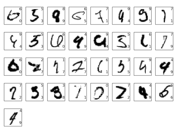
Some Failures
*Not from this particular network