Computer Systems Overview

1/28/2026

print view

%%html
<script src="https://bits.csb.pitt.edu/preamble.js"></script>

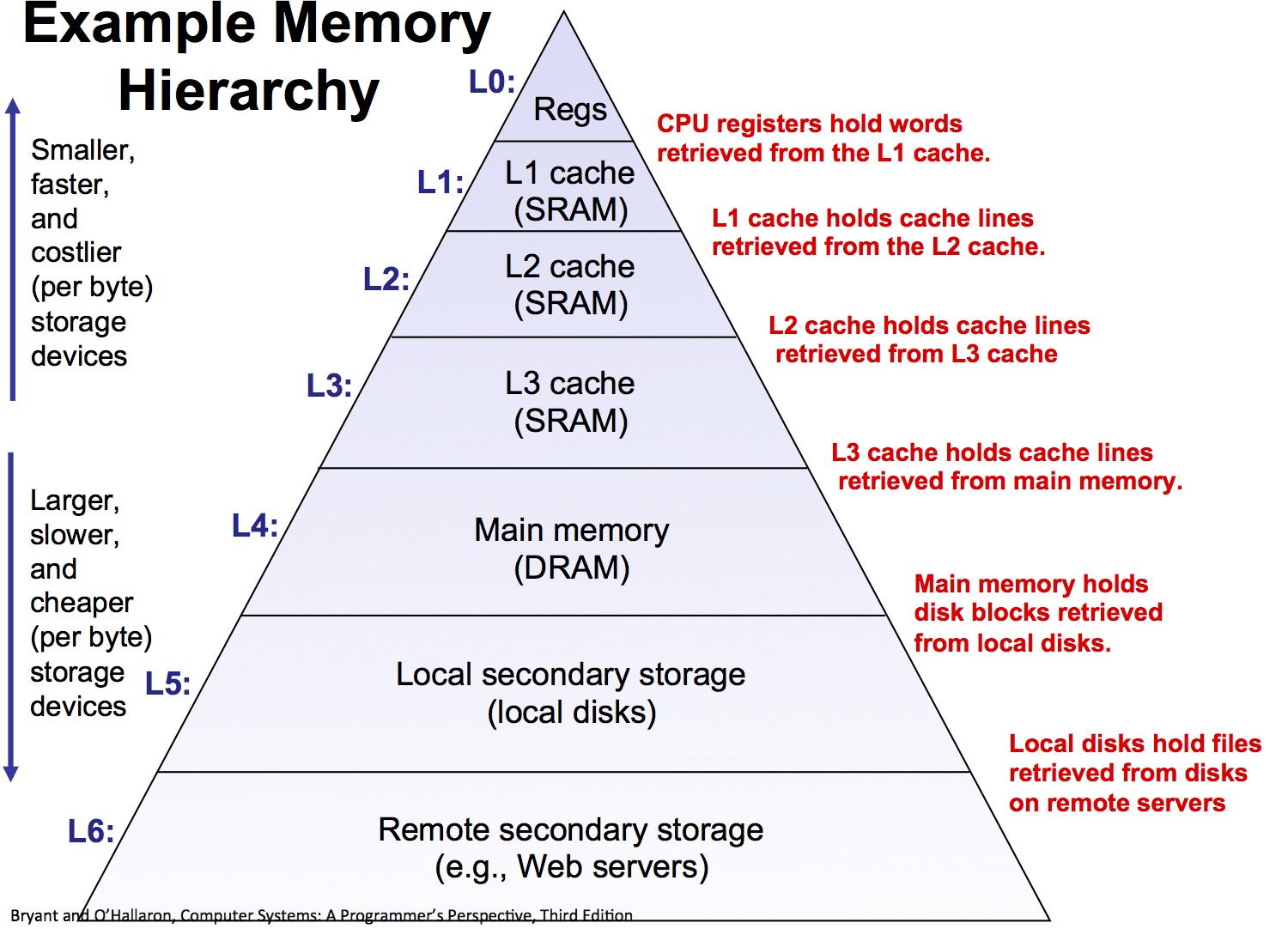
Memory Access Times

• L1 Cache 1-2ns
• L2 Cache 3-5ns
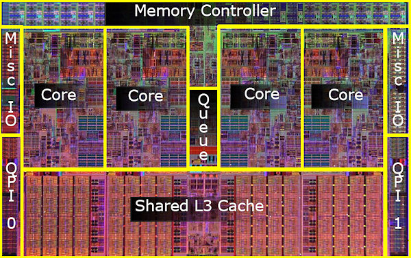
• L3 Cache 12-20ns
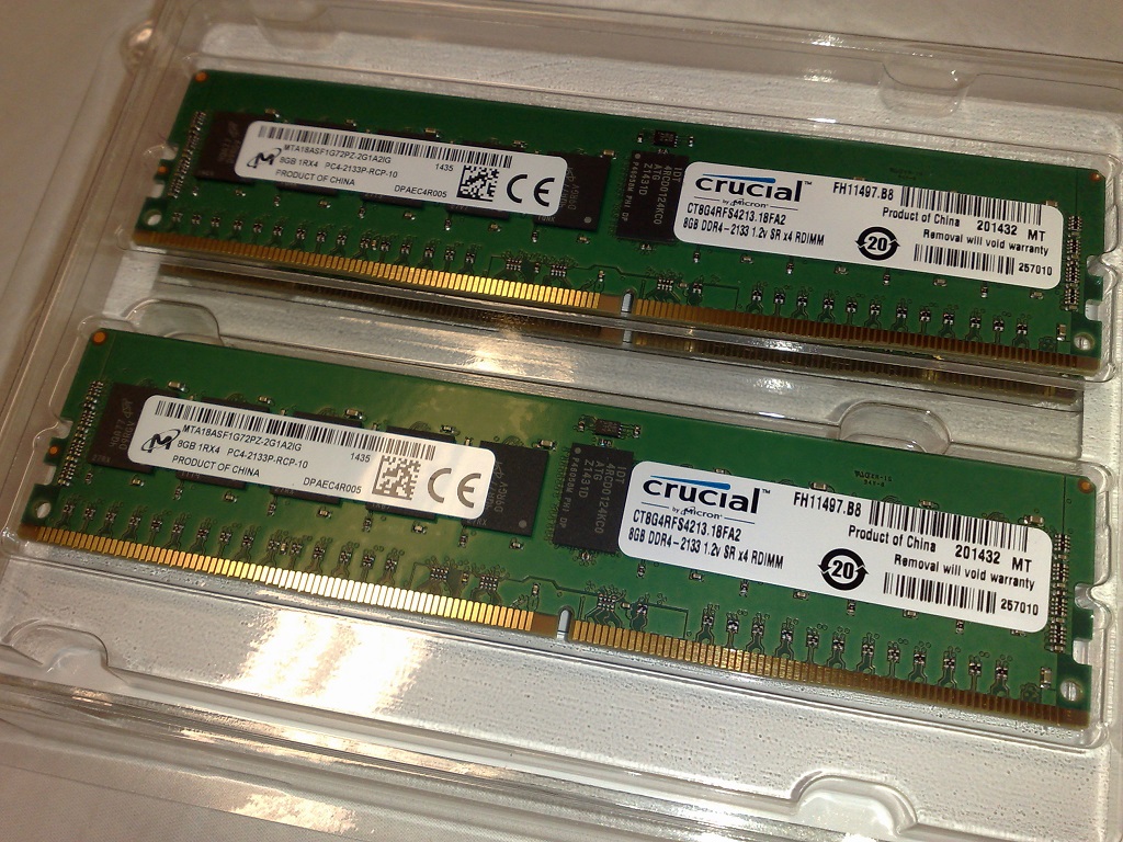
• DRAM 60-200ns

Memory througput (sequential): 8-400 GB/s (GPUs even higher)

Disk Access Time

Seek time: 8-12ms

Sequential read throughput: ~50-300MB/s

Random read throughput: < 1MB/s

Cost: \$0.01/GB - $0.10/GB

Disks kill random-access workloads

SSD Access Time

Access time: 5-50$\mu$s

Sequential read throughput: 500 - 3500MB/s

Random read throughput: 25-50MB/s (but improves 10-20X if requests done simultaneously)

Cost: \$0.05/GB - $0.20/GB

%%html
<div id="mlaccess" style="width: 500px"></div>
<script>
$('head').append('<link rel="stylesheet" href="https://bits.csb.pitt.edu/asker.js/themes/asker.default.css" />');


	jQuery('#mlaccess').asker({
	    id: "mlaccess",
	    question: "How much faster is it to access memory than disk?",
		answers: ["100X","1,000X","10,000X","100,000X","1,000,000X"],
        server: "https://bits.csb.pitt.edu/asker.js/example/asker.cgi",
		charter: chartmaker})
    
$(".jp-InputArea .o:contains(html)").closest('.jp-InputArea').hide();


</script>

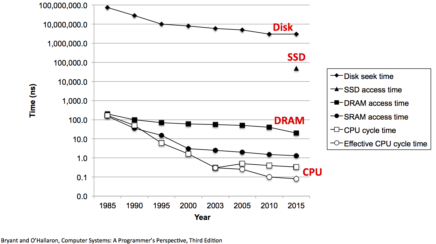
Takeaways

• Disks are slow compared to memory. Really slow (even SSDs)

• But they are still the most cost effective means of storing large datasets

• Memory hierarchies use caching to exploit locality and provide high-speed access to large datasets.

Parallel Programming

There are several parallel programming models enabled by a variety of hardware (multicore, cloud computing, supercomputers, GPU).

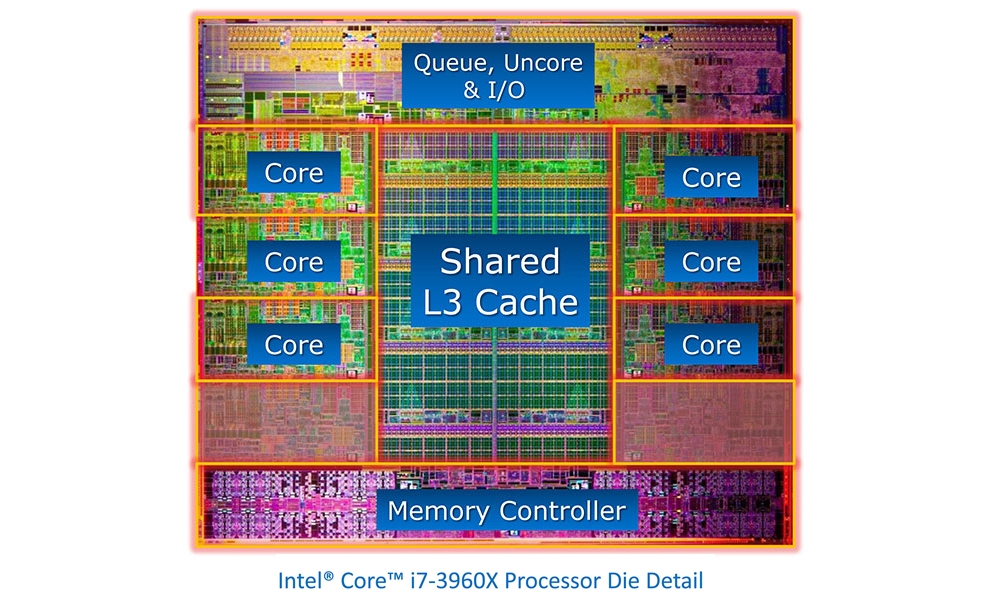
Threads vs. Processes

A thread of execution is the smallest sequence of programmed instructions that can be managed independently by an operating system scheduler.

A process is an instance of a computer program.

Address Spaces

A process has its own address space. An address space is a mapping of virtual memory addresses to physical memory addresses managed by the operating system.

Address spaces prevent processes from crashing other applications or the operating system - they can only access their own memory.

Threads vs. Processs

import threading,time

cnt = [0]

def incrementCnt(cnt):
    for i in range(1000000): # a million times
        x = cnt[0] 

t1 = threading.Thread(target=incrementCnt,args=(cnt,))
t2 = threading.Thread(target=incrementCnt,args=(cnt,))

t1.start()
t2.start()

What do we expect when we print cnt?

%%html
<div id="mlthread1" style="width: 500px"></div>
<script>
$('head').append('<link rel="stylesheet" href="https://bits.csb.pitt.edu/asker.js/themes/asker.default.css" />');

    var divid = '#mlthread1';
	jQuery(divid).asker({
	    id: divid,
	    question: "What is cnt?",
		answers: ['0','2','1000000','2000000',"I don't know"],
        server: "https://bits.csb.pitt.edu/asker.js/example/asker.cgi",
		charter: chartmaker})
    
$(".jp-InputArea .o:contains(html)").closest('.jp-InputArea').hide();

</script>

The Answer

import threading,time

cnt = [0]

def incrementCnt(cnt):
    for i in range(1000000): # a million times
        cnt[0] += 1

t1 = threading.Thread(target=incrementCnt,args=(cnt,))
t2 = threading.Thread(target=incrementCnt,args=(cnt,))
t1.start()
t2.start()

print(cnt) #what do we expect to print out?
time.sleep(1)
print(cnt)
time.sleep(1)
print(cnt)

[6446]
[2000000]
[2000000]

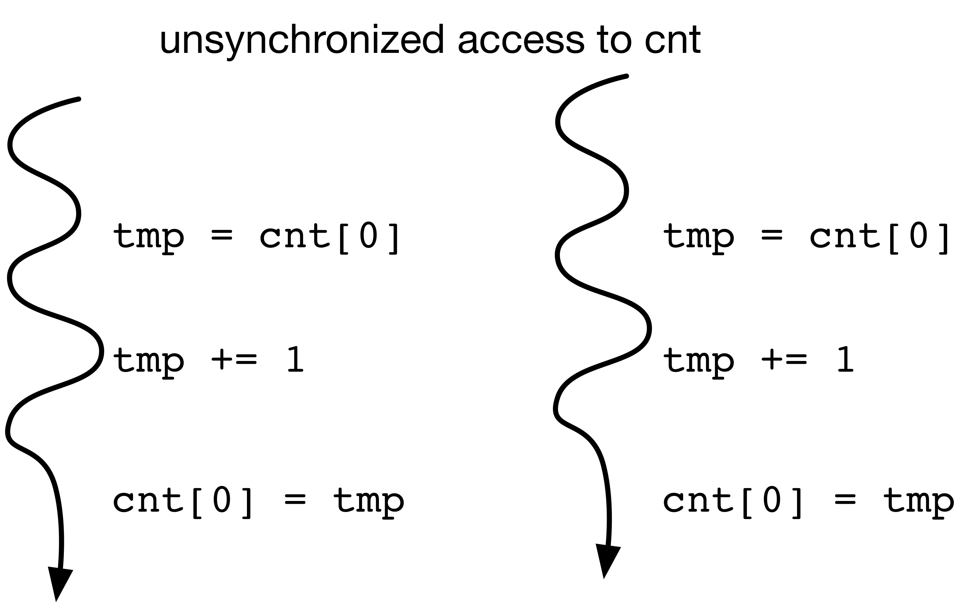
import threading,time

cnt = [0]

def incrementCnt(cnt):
    for i in range(10000): # a million times
        x = cnt[0]
        x += 1
        time.sleep(0)
        cnt[0] = x

t1 = threading.Thread(target=incrementCnt,args=(cnt,))
t2 = threading.Thread(target=incrementCnt,args=(cnt,))
t1.start()
t2.start()

print(cnt) #what do we expect to print out?
time.sleep(1)
print(cnt)
time.sleep(1)

print(cnt)

[2]
[10002]
[10002]

Threads vs. Processes

import multiprocess,time

cnt = [0]

p1 = multiprocess.Process(target=incrementCnt,args=(cnt,))
p2 = multiprocess.Process(target=incrementCnt,args=(cnt,))

p1.start()
p2.start()

#what do we expect when we print out cnt[0]?

%%html
<div id="mlproc1" style="width: 500px"></div>
<script>
$('head').append('<link rel="stylesheet" href="https://bits.csb.pitt.edu/asker.js/themes/asker.default.css" />');

    var divid = '#mlproc1';
	jQuery(divid).asker({
	    id: divid,
	    question: "What will print out?",
		answers: ['0','2','1000000','2000000',"I don't know"],
        server: "https://bits.csb.pitt.edu/asker.js/example/asker.cgi",
		charter: chartmaker})
    
$(".jp-InputArea .o:contains(html)").closest('.jp-InputArea').hide();


</script>

The Answer

cnt = [0]
p1 = multiprocess.Process(target=incrementCnt,args=(cnt,))
p2 = multiprocess.Process(target=incrementCnt,args=(cnt,))

p1.start()
p2.start()

print(cnt[0])
time.sleep(3)
print(cnt[0])

0
0

Parallel Programming Concepts: Communication

Threads can communicate through their shared address space using locks to protect sensitive state (e.g., ensure data is updated atomically). However, using simpler, less flexible communication protocols makes it easier to write correct code.

Queue

Provides one-way communication between many threads/processes (producer-consumer)

Pipe/Socket

Provides two-way communication between two threads/processes

These are examples of communication with message passing.

Queue Example

def dowork(inQ, outQ):
    val = inQ.get()
    outQ.put(val*val)

inQ = multiprocess.Queue()
outQ = multiprocess.Queue()
pool = multiprocess.Pool(4, dowork, (inQ, outQ))

inQ.put(4)

outQ.get()

16

Pipe Example

import multiprocess

def chatty(conn): #this takes a Connection object representing one end of a pipe
    msg = conn.recv()
    conn.send("you sent me "+msg)
    
(c1,c2) = multiprocess.Pipe()

p1 = multiprocess.Process(target=chatty,args=(c2,))
p1.start()

c1.send("Hello!")
result = c1.recv()
p1.join()

print(result)

you sent me Hello!

Pools

multiprocess supports the concept of a pool of workers. You initialize with the number of processes you want to run in parallel (the default is the number of CPUs on your system) and they are available for doing parallel work:

• map: the most important function - just like the built-in map, this will map a function to an iterable and return the result, but the mapping will be done in parallel. Blocks until the full result is computed and the result is in the proper order.
• map_async: map without blocking
• imap: parallel imap - returns iterable instead of list. The next() method of the returned iterable will block if necessary.
• imap_unordered: same as imap but returns values in order they are computed
• close: close the pool to prevent additional jobs from being submitted
• join: must call close first; waits for all jobs to complete

Pool Example

def f(x):
    return x*x

pool = multiprocess.Pool(processes=4)

print(pool.map(f,range(20)))

[0, 1, 4, 9, 16, 25, 36, 49, 64, 81, 100, 121, 144, 169, 196, 225, 256, 289, 324, 361]

Threads or Processes?

Normally, the choice between threads and processes depends on how data will be accessed and the level of communication between parallel tasks etc.

However, in Python, the answer is almost always use multiprocessing, not threading.

Why? The CPython interpretter has a Global Interpretter Lock. This means that only one thread of python code is actually executed at any given time when using threads. With processes, each process has its own interpretter (with its own lock).

The main issue with processes is you have to copy data between address spaces.

Memory Mapping

Multiple virtual addresses can map to the same physical address. This is especially useful for read-only data.

Virtual addresses need not map to physical addresses - they can also be placeholders to indicate the data is stored elsewhere.

Swapping The operating system can move data from memory to disk (swap it out) if it needs more memory. When the corresponding virtual address is accessed a page fault occurs and the data is loaded back from disk into memory.

When mmap can provide performance benefit

• Your data can be stored in a single local file
• Your data is read only
• The size of the data does not fit comfortably in memory or N processes will use the same data and N copies does not fit comfortably in memory
• You need to read the data more than once
  • If only need to read once, optimize for sequential access and stream it
• Data is not accessed sequentially
• Your code will run on machines with different amounts of available memory

In a memory limited situation, mmapping will be substantially faster than reading directly into memory. Why?

lmdb

Lightning Memory-Mapped Database. https://lmdb.readthedocs.io/en/release/

(key,value) pairs of bytestrings

import lmdb

env = lmdb.open('db')
with env.begin(write=True) as txn:
    txn.put(b'key1',b'123')
    txn.put(b'key2',b'abc')

env = lmdb.open('db',readonly=True)
with env.begin() as txn:
    print(txn.get(b'key1'))

b'123'

Going beyond raw bytes

import numpy as np
a = np.array([1.0,3.14,2])
env = lmdb.open('db')
with env.begin(write=True) as txn:
    txn.put(b'key', a)

env = lmdb.open('db',readonly=True)
with env.begin() as txn:
    buffer = txn.get(b'key')
buffer

b'\x00\x00\x00\x00\x00\x00\xf0?\x1f\x85\xebQ\xb8\x1e\t@\x00\x00\x00\x00\x00\x00\x00@'

newa = np.frombuffer(buffer,dtype=np.float64) # does NOT copy!

newa.base is buffer

True

newa[0] = 4

---------------------------------------------------------------------------
ValueError                                Traceback (most recent call last)
Cell In[52], line 1
----> 1 newa[0] = 4

ValueError: assignment destination is read-only

HDF5

• "self-describing" framework for defining a binary format
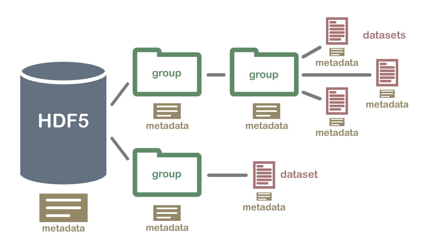
• datasets organized into (possibly nested) groups
• dataset has type, dataspace (layout), properties, and annotations in addition to data

Specializations of HDF5

• netcdf4 - (array data) is implemented on top of HDF5
• anndata - annotated data (https://anndata.readthedocs.io/)

AnnData

import h5py  # tries to provide numpy interface to hd5 data

mouse = h5py.File('mouse_tabula_muris_10x_log1p_cpm.h5ad','r')

mouse.keys()

<KeysViewHDF5 ['X', 'obs', 'raw.X', 'raw.var', 'uns', 'var']>

mouse['obs']  # "opaque" type of size 45

<HDF5 dataset "obs": shape (54967,), type "|V45">

np.array(mouse['obs'])

array([(b'10X_P4_0_AAACCTGAGATTACCC', 10, 2,  7, 0.11555646,  9848., 2857),
       (b'10X_P4_0_AAACCTGAGTGCCAGA', 10, 2, 31, 0.17775837, 17175., 2933),
       (b'10X_P4_0_AAACCTGCAAATCCGT', 10, 2, 31, 0.09034352, 22181., 3217),
       ...,
       (b'10X_P8_15_TTTGTCATCGGCTTGG', 11, 2, 19, 0.09656238,  2589., 1302),
       (b'10X_P8_15_TTTGTCATCTTACCGC', 11, 2, 44, 0.10493047,  2373.,  973),
       (b'10X_P8_15_TTTGTCATCTTGTTTG', 11, 2, 44, 0.07301372,  5903., 1800)],
      dtype=[('index', 'S26'), ('tissue', 'i1'), ('subtissue', 'i1'), ('cell_ontology_class', 'i1'), ('percent_ribo', '<f4'), ('n_counts', '<f4'), ('n_genes', '<i8')])

import pandas as pd
pd.DataFrame(np.array(mouse['obs']))

	index	tissue	subtissue	cell_ontology_class	percent_ribo	n_counts	n_genes
0	b'10X_P4_0_AAACCTGAGATTACCC'	10	2	7	0.115556	9848.0	2857
1	b'10X_P4_0_AAACCTGAGTGCCAGA'	10	2	31	0.177758	17175.0	2933
2	b'10X_P4_0_AAACCTGCAAATCCGT'	10	2	31	0.090344	22181.0	3217
3	b'10X_P4_0_AAACCTGGTAATCGTC'	10	2	7	0.185273	16840.0	3108
4	b'10X_P4_0_AAACCTGGTCCAACTA'	10	2	7	0.144283	19531.0	3713
...	...	...	...	...	...	...	...
54962	b'10X_P8_15_TTTGTCAGTTGTCGCG'	11	2	19	0.126633	6507.0	2256
54963	b'10X_P8_15_TTTGTCATCACGATGT'	11	2	11	0.128589	1672.0	772
54964	b'10X_P8_15_TTTGTCATCGGCTTGG'	11	2	19	0.096562	2589.0	1302
54965	b'10X_P8_15_TTTGTCATCTTACCGC'	11	2	44	0.104930	2373.0	973
54966	b'10X_P8_15_TTTGTCATCTTGTTTG'	11	2	44	0.073014	5903.0	1800

54967 rows × 7 columns

mouse['var']

<HDF5 dataset "var": shape (18099,), type "|V22">

mouse['var'].dtype

dtype([('index', 'S14'), ('n_cells', '<i8')])

np.array(mouse['var'])

array([(b'0610005C13Rik',  1847), (b'0610007C21Rik', 23434),
       (b'0610007L01Rik', 13040), ..., (b'Zzz3',  8077), (b'a',   165),
       (b'l7Rn6', 14131)], dtype=[('index', 'S14'), ('n_cells', '<i8')])

import pandas as pd
pd.DataFrame(np.array(mouse['var']))

	index	n_cells
0	b'0610005C13Rik'	1847
1	b'0610007C21Rik'	23434
2	b'0610007L01Rik'	13040
3	b'0610007N19Rik'	11829
4	b'0610007P08Rik'	3299
...	...	...
18094	b'Zyx'	18955
18095	b'Zzef1'	6096
18096	b'Zzz3'	8077
18097	b'a'	165
18098	b'l7Rn6'	14131

18099 rows × 2 columns

mouse['X']

<HDF5 group "/X" (3 members)>

mouse['X'].keys()

<KeysViewHDF5 ['data', 'indices', 'indptr']>

dict(mouse['X'].attrs)

{'h5sparse_format': 'csr', 'h5sparse_shape': array([54967, 18099])}

mouse['X']['data']

<HDF5 dataset "data": shape (105321967,), type "<f4">

This is a sparse matrix representation (compressed sparse row)

$$54967×18099 = 994,847,733 >> 105,321,967$$

import scipy.sparse
X = mouse['X']
M = scipy.sparse.csr_matrix((X['data'],X['indices'],X['indptr']))

M

<54967x18099 sparse matrix of type '<class 'numpy.float32'>'
	with 105321967 stored elements in Compressed Sparse Row format>

mouse['uns'].keys()

<KeysViewHDF5 ['cell_ontology_class_categories', 'subtissue_categories', 'tissue_categories']>

np.array(mouse['uns']['cell_ontology_class_categories'])

array([b'B cell', b'DN1 thymic pro-T cell', b'Fraction A pre-pro B cell',
       b'Langerhans cell', b'T cell', b'alveolar macrophage',
       b'basal cell', b'basal cell of epidermis', b'basophil',
       b'bladder cell', b'bladder urothelial cell', b'blood cell',
       b'cardiac muscle cell',
       b'ciliated columnar cell of tracheobronchial tree',
       b'classical monocyte', b'dendritic cell', b'duct epithelial cell',
       b'early pro-B cell', b'endocardial cell', b'endothelial cell',
       b'endothelial cell of hepatic sinusoid', b'epithelial cell',
       b'erythroblast', b'erythrocyte', b'fibroblast', b'granulocyte',
       b'granulocytopoietic cell', b'hematopoietic precursor cell',
       b'hepatocyte', b'immature B cell', b'immature T cell',
       b'keratinocyte', b'kidney capillary endothelial cell',
       b'kidney cell', b'kidney collecting duct epithelial cell',
       b'kidney loop of Henle ascending limb epithelial cell',
       b'kidney proximal straight tubule epithelial cell',
       b'late pro-B cell', b'leukocyte',
       b'luminal epithelial cell of mammary gland',
       b'lung endothelial cell', b'macrophage', b'mast cell',
       b'mesangial cell', b'mesenchymal cell', b'mesenchymal stem cell',
       b'monocyte', b'myeloid cell', b'natural killer cell',
       b'neuroendocrine cell', b'non-classical monocyte',
       b'proerythroblast', b'professional antigen presenting cell',
       b'promonocyte', b'skeletal muscle satellite cell', b'stromal cell',
       b'type II pneumocyte'], dtype=object)

anndata package provides a higher level interface

import anndata
data = anndata.read_h5ad('mouse_tabula_muris_10x_log1p_cpm.h5ad')
data

AnnData object with n_obs × n_vars = 54967 × 18099
    obs: 'tissue', 'subtissue', 'cell_ontology_class', 'percent_ribo', 'n_counts', 'n_genes'
    var: 'n_cells'

data.obs

	tissue	subtissue	cell_ontology_class	percent_ribo	n_counts	n_genes
index
10X_P4_0_AAACCTGAGATTACCC	Tongue	nan	basal cell of epidermis	0.115556	9848.0	2857
10X_P4_0_AAACCTGAGTGCCAGA	Tongue	nan	keratinocyte	0.177758	17175.0	2933
10X_P4_0_AAACCTGCAAATCCGT	Tongue	nan	keratinocyte	0.090344	22181.0	3217
10X_P4_0_AAACCTGGTAATCGTC	Tongue	nan	basal cell of epidermis	0.185273	16840.0	3108
10X_P4_0_AAACCTGGTCCAACTA	Tongue	nan	basal cell of epidermis	0.144283	19531.0	3713
...	...	...	...	...	...	...
10X_P8_15_TTTGTCAGTTGTCGCG	Trachea	nan	endothelial cell	0.126633	6507.0	2256
10X_P8_15_TTTGTCATCACGATGT	Trachea	nan	blood cell	0.128589	1672.0	772
10X_P8_15_TTTGTCATCGGCTTGG	Trachea	nan	endothelial cell	0.096562	2589.0	1302
10X_P8_15_TTTGTCATCTTACCGC	Trachea	nan	mesenchymal cell	0.104930	2373.0	973
10X_P8_15_TTTGTCATCTTGTTTG	Trachea	nan	mesenchymal cell	0.073014	5903.0	1800

54967 rows × 6 columns

scanpy - anndata wrapper specifically for single cell data

import scanpy
data=scanpy.read_h5ad('mouse_tabula_muris_10x_log1p_cpm.h5ad')

data

AnnData object with n_obs × n_vars = 54967 × 18099
    obs: 'tissue', 'subtissue', 'cell_ontology_class', 'percent_ribo', 'n_counts', 'n_genes'
    var: 'n_cells'

data.var_names

Index(['0610005C13Rik', '0610007C21Rik', '0610007L01Rik', '0610007N19Rik',
       '0610007P08Rik', '0610007P14Rik', '0610007P22Rik', '0610008F07Rik',
       '0610009B14Rik', '0610009B22Rik',
       ...
       'Zxda', 'Zxdb', 'Zxdc', 'Zyg11a', 'Zyg11b', 'Zyx', 'Zzef1', 'Zzz3', 'a',
       'l7Rn6'],
      dtype='object', name='index', length=18099)

data.var

	n_cells
index
0610005C13Rik	1847
0610007C21Rik	23434
0610007L01Rik	13040
0610007N19Rik	11829
0610007P08Rik	3299
...	...
Zyx	18955
Zzef1	6096
Zzz3	8077
a	165
l7Rn6	14131

18099 rows × 1 columns

data.X

<54967x18099 sparse matrix of type '<class 'numpy.float32'>'
	with 105321967 stored elements in Compressed Sparse Row format>

data.X[:5,:5]

<5x5 sparse matrix of type '<class 'numpy.float32'>'
	with 6 stored elements in Compressed Sparse Row format>

data.X[:5,:5].toarray()

array([[0.       , 5.7223763, 0.       , 0.       , 5.318546 ],
       [0.       , 4.08133  , 4.08133  , 0.       , 0.       ],
       [0.       , 4.914498 , 0.       , 0.       , 0.       ],
       [0.       , 0.       , 0.       , 0.       , 0.       ],
       [0.       , 3.955095 , 0.       , 0.       , 0.       ]],
      dtype=float32)

data.obs

	tissue	subtissue	cell_ontology_class	percent_ribo	n_counts	n_genes
index
10X_P4_0_AAACCTGAGATTACCC	Tongue	nan	basal cell of epidermis	0.115556	9848.0	2857
10X_P4_0_AAACCTGAGTGCCAGA	Tongue	nan	keratinocyte	0.177758	17175.0	2933
10X_P4_0_AAACCTGCAAATCCGT	Tongue	nan	keratinocyte	0.090344	22181.0	3217
10X_P4_0_AAACCTGGTAATCGTC	Tongue	nan	basal cell of epidermis	0.185273	16840.0	3108
10X_P4_0_AAACCTGGTCCAACTA	Tongue	nan	basal cell of epidermis	0.144283	19531.0	3713
...	...	...	...	...	...	...
10X_P8_15_TTTGTCAGTTGTCGCG	Trachea	nan	endothelial cell	0.126633	6507.0	2256
10X_P8_15_TTTGTCATCACGATGT	Trachea	nan	blood cell	0.128589	1672.0	772
10X_P8_15_TTTGTCATCGGCTTGG	Trachea	nan	endothelial cell	0.096562	2589.0	1302
10X_P8_15_TTTGTCATCTTACCGC	Trachea	nan	mesenchymal cell	0.104930	2373.0	973
10X_P8_15_TTTGTCATCTTGTTTG	Trachea	nan	mesenchymal cell	0.073014	5903.0	1800

54967 rows × 6 columns