Deep Learning: A Recurrent Topic

2/22/2024

print view

%%html
<script src="https://bits.csb.pitt.edu/preamble.js"></script>

Recall - PyTorch Network

X = 2304

import torch
import torch.nn as nn
import torch.nn.functional as F
import numpy as np
import matplotlib.pyplot as plt
%matplotlib inline

class MyNet(nn.Module):
    def __init__(self):  #initialize submodules here - this defines our network architecture
        super(MyNet, self).__init__()
        self.conv1 = nn.Conv2d(in_channels=1, out_channels=32, kernel_size=3, stride=1, padding=1) 
        self.conv2 = nn.Conv2d(in_channels=32, out_channels=64, kernel_size=3, stride=1)
        self.fc1 = nn.Linear(2304, 10) #mystery X is 2304

    def forward(self, x): # this actually applies the operations
        x = self.conv1(x)
        x = F.relu(x)
        x = F.max_pool2d(x, kernel_size=2, stride=2)  # POOL    
        x = self.conv2(x)
        x = F.relu(x)
        x = F.max_pool2d(x, kernel_size=2, stride=2) # POOL
        x = torch.flatten(x, 1)
        x = self.fc1(x)
        return x

MNIST

from torchvision import datasets
train_data = datasets.MNIST(root='../data', train=True,download=True)
test_data = datasets.MNIST(root='../data', train=False,download=True)

Dataset

Either map-style or iterable

• map-style Implements __getitem__ and __len__. Single data item is accessed dataset[idx]
• iterable-style Implements __iter__ for sequential traversal of data

train_data[0]

(<PIL.Image.Image image mode=L size=28x28 at 0x7F38F45DA020>, 5)

train_data[0][0]

Inputs need to be tensors...

from torchvision import transforms
train_data = datasets.MNIST(root='../data', train=True,transform=transforms.ToTensor())
test_data = datasets.MNIST(root='../data', train=False,transform=transforms.ToTensor())

Custom Dataset

import os
import pandas as pd
from torchvision.io import read_image
from torch.utils.data import Dataset

class CustomImageDataset(Dataset):
    def __init__(self, annotations_file, img_dir, transform=None, target_transform=None):
        self.img_labels = pd.read_csv(annotations_file)
        self.img_dir = img_dir
        self.transform = transform
        self.target_transform = target_transform

    def __len__(self):
        return len(self.img_labels)

    def __getitem__(self, idx):
        img_path = os.path.join(self.img_dir, self.img_labels.iloc[idx, 0])
        image = read_image(img_path)
        label = self.img_labels.iloc[idx, 1]
        if self.transform:
            image = self.transform(image)
        if self.target_transform:
            label = self.target_transform(label)
        return image, label

Training MNIST

#process 10 randomly sampled images at a time
train_loader = torch.utils.data.DataLoader(train_data,batch_size=10,shuffle=True,num_workers=8)
test_loader = torch.utils.data.DataLoader(test_data,batch_size=10,shuffle=False)

DataLoader

• customize data loading order (e.g. shuffle)
• automatic batching
• multi-process data loading, prefetching

batch = next(iter(train_loader))
batch

[tensor([[[[0., 0., 0.,  ..., 0., 0., 0.],
           [0., 0., 0.,  ..., 0., 0., 0.],
           [0., 0., 0.,  ..., 0., 0., 0.],
           ...,
           [0., 0., 0.,  ..., 0., 0., 0.],
           [0., 0., 0.,  ..., 0., 0., 0.],
           [0., 0., 0.,  ..., 0., 0., 0.]]],
 
 
         [[[0., 0., 0.,  ..., 0., 0., 0.],
           [0., 0., 0.,  ..., 0., 0., 0.],
           [0., 0., 0.,  ..., 0., 0., 0.],
           ...,
           [0., 0., 0.,  ..., 0., 0., 0.],
           [0., 0., 0.,  ..., 0., 0., 0.],
           [0., 0., 0.,  ..., 0., 0., 0.]]],
 
 
         [[[0., 0., 0.,  ..., 0., 0., 0.],
           [0., 0., 0.,  ..., 0., 0., 0.],
           [0., 0., 0.,  ..., 0., 0., 0.],
           ...,
           [0., 0., 0.,  ..., 0., 0., 0.],
           [0., 0., 0.,  ..., 0., 0., 0.],
           [0., 0., 0.,  ..., 0., 0., 0.]]],
 
 
         ...,
 
 
         [[[0., 0., 0.,  ..., 0., 0., 0.],
           [0., 0., 0.,  ..., 0., 0., 0.],
           [0., 0., 0.,  ..., 0., 0., 0.],
           ...,
           [0., 0., 0.,  ..., 0., 0., 0.],
           [0., 0., 0.,  ..., 0., 0., 0.],
           [0., 0., 0.,  ..., 0., 0., 0.]]],
 
 
         [[[0., 0., 0.,  ..., 0., 0., 0.],
           [0., 0., 0.,  ..., 0., 0., 0.],
           [0., 0., 0.,  ..., 0., 0., 0.],
           ...,
           [0., 0., 0.,  ..., 0., 0., 0.],
           [0., 0., 0.,  ..., 0., 0., 0.],
           [0., 0., 0.,  ..., 0., 0., 0.]]],
 
 
         [[[0., 0., 0.,  ..., 0., 0., 0.],
           [0., 0., 0.,  ..., 0., 0., 0.],
           [0., 0., 0.,  ..., 0., 0., 0.],
           ...,
           [0., 0., 0.,  ..., 0., 0., 0.],
           [0., 0., 0.,  ..., 0., 0., 0.],
           [0., 0., 0.,  ..., 0., 0., 0.]]]]),
 tensor([0, 5, 3, 4, 2, 1, 0, 7, 8, 1])]

Model

#instantiate our neural network and put it on the GPU
model = MyNet().to('cuda')

Training MNIST

%%time
optimizer = torch.optim.Adam(model.parameters(), lr=0.00001) # need to tell optimizer what it is optimizing

losses = []
for epoch in range(10):
    for i, (img,label) in enumerate(train_loader):
        optimizer.zero_grad()  # IMPORTANT!        
        img, label = img.to('cuda'), label.to('cuda')
        output = model(img)
        loss = F.cross_entropy(output, label)
        loss.backward()
        optimizer.step()
        losses.append(loss.item())

CPU times: user 2min 15s, sys: 13.4 s, total: 2min 29s
Wall time: 2min 45s

Testing MNIST

correct = 0
with torch.no_grad(): #no need for gradients - won't be calling backward to clear them
    for img, label in test_loader:
        img, label = img.to('cuda'), label.to('cuda')
        output = F.softmax(model(img),dim=1)
        pred = output.argmax(dim=1, keepdim=True)  # get the index of the max log-probability
        correct += pred.eq(label.view_as(pred)).sum().item()
        
print("Accuracy",correct/len(test_loader.dataset))

Accuracy 0.9695

Batch Normalization

Normalize input based on batch statistics to have zero mean and unit variance.

https://arxiv.org/abs/1502.03167

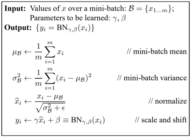
Batch Normalization

• Used throughout network
• Reduces "internal covariate shift"
• Less sensitive to weight initialization
• Can use higher learning rates
• Acts as regularizer
• At test time typically uses running average/variance calculated during training

class MyBNNet(nn.Module):
    def __init__(self):  #initialize submodules here - this defines our network architecture
        super(MyBNNet, self).__init__()
        self.conv1 = nn.Conv2d(in_channels=1, out_channels=32, kernel_size=3, stride=1, padding=1) 
        self.bn1 = nn.BatchNorm2d(32)
        self.conv2 = nn.Conv2d(in_channels=32, out_channels=64, kernel_size=3, stride=1)
        self.bn2 = nn.BatchNorm2d(64)
        self.fc1 = nn.Linear(X, 10) #mystery X

    def forward(self, x): # this actually applies the operations
        x = self.conv1(x)
        x = self.bn1(x)
        x = F.relu(x)
        x = F.max_pool2d(x, kernel_size=2, stride=2)  # POOL    
        x = self.conv2(x)
        x = self.bn2(x)
        x = F.relu(x)
        x = F.max_pool2d(x, kernel_size=2, stride=2) # POOL
        x = torch.flatten(x, 1)
        x = self.fc1(x)
        return x
    
#instantiate our neural network and put it on the GPU
bnmodel = MyBNNet().to('cuda')    

%%html
<div id="bnq" style="width: 500px"></div>
<script>

    var divid = '#bnq';
	jQuery(divid).asker({
	    id: divid,
	    question: "Does BatchNorm2d have learned parameters?",
		answers: ["Yes","No"],
        server: "https://bits.csb.pitt.edu/asker.js/example/asker.cgi",
		charter: chartmaker})
    
$(".jp-InputArea .o:contains(html)").closest('.jp-InputArea').hide();

</script>

list(nn.BatchNorm2d(32).parameters())

[Parameter containing:
 tensor([1., 1., 1., 1., 1., 1., 1., 1., 1., 1., 1., 1., 1., 1., 1., 1., 1., 1.,
         1., 1., 1., 1., 1., 1., 1., 1., 1., 1., 1., 1., 1., 1.],
        requires_grad=True),
 Parameter containing:
 tensor([0., 0., 0., 0., 0., 0., 0., 0., 0., 0., 0., 0., 0., 0., 0., 0., 0., 0., 0., 0., 0., 0., 0., 0.,
         0., 0., 0., 0., 0., 0., 0., 0.], requires_grad=True)]

%%time
optimizer = torch.optim.Adam(bnmodel.parameters(), lr=0.00001) # need to tell optimizer what it is optimizing

losses = []
for epoch in range(10):
    for i, (img,label) in enumerate(train_loader):
        optimizer.zero_grad()  # IMPORTANT!        
        img, label = img.to('cuda'), label.to('cuda')
        output = bnmodel(img)
        loss = F.cross_entropy(output, label)
        loss.backward()
        optimizer.step()
        losses.append(loss.item())

CPU times: user 2min 43s, sys: 14.9 s, total: 2min 58s
Wall time: 3min 16s

list(bnmodel.bn1.parameters())

[Parameter containing:
 tensor([1.0372, 0.9922, 0.9809, 0.9748, 0.9933, 0.9921, 0.9806, 1.0521, 0.9749,
         1.0243, 0.9782, 0.9941, 1.0215, 0.9868, 0.9966, 1.0007, 1.0545, 1.0079,
         1.0125, 0.9868, 1.0072, 0.9811, 1.0127, 0.9957, 1.0211, 0.9882, 1.0116,
         0.9805, 1.0416, 1.0007, 1.0583, 0.9992], device='cuda:0',
        requires_grad=True),
 Parameter containing:
 tensor([ 0.0257,  0.0112, -0.0017, -0.0206, -0.0091, -0.0049, -0.0288,  0.0109,
         -0.0055, -0.0064, -0.0418, -0.0267, -0.0114, -0.0163, -0.0101, -0.0199,
          0.0154, -0.0003, -0.0136,  0.0001, -0.0133, -0.0337,  0.0007, -0.0343,
          0.0112, -0.0217, -0.0050, -0.0018, -0.0045, -0.0231,  0.0045, -0.0051],
        device='cuda:0', requires_grad=True)]

correct = 0
with torch.no_grad(): #no need for gradients - won't be calling backward to clear them
    for img, label in test_loader:
        img, label = img.to('cuda'), label.to('cuda')
        output = F.softmax(bnmodel(img),dim=1)
        pred = output.argmax(dim=1, keepdim=True)  # get the index of the max log-probability
        correct += pred.eq(label.view_as(pred)).sum().item()
        
print("Accuracy",correct/len(test_loader.dataset))

Accuracy 0.9856

That was wrong!

correct = 0
bnmodel.eval() # NEED TO PUT IN EVAL MODE!
with torch.no_grad(): #no need for gradients - won't be calling backward to clear them
    for img, label in test_loader:
        img, label = img.to('cuda'), label.to('cuda')
        output = F.softmax(bnmodel(img),dim=1)
        pred = output.argmax(dim=1, keepdim=True)  # get the index of the max log-probability
        correct += pred.eq(label.view_as(pred)).sum().item()
        
print("Accuracy",correct/len(test_loader.dataset))

Accuracy 0.985

Deep Learning Architectures

https://adeshpande3.github.io/adeshpande3.github.io/The-9-Deep-Learning-Papers-You-Need-To-Know-About.html

GoogLeNet (2014)

More than 100 layers

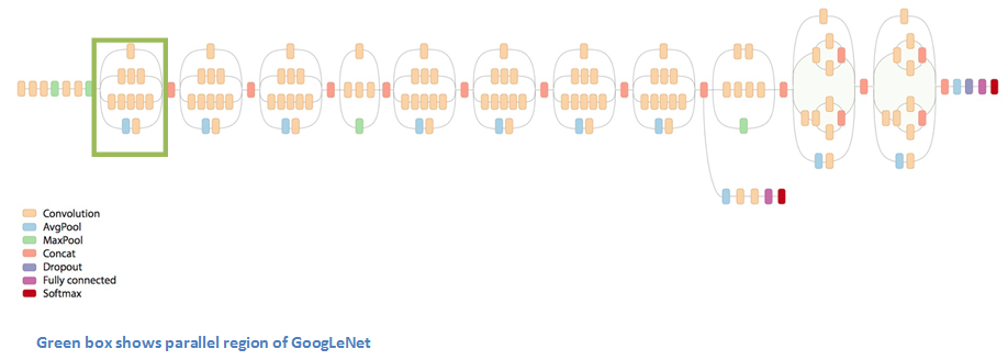
GoogLeNet - Inception Module

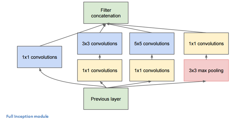
"Network in network" - 1D convolutional layers that reduce the number of filters.

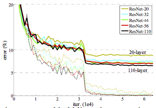
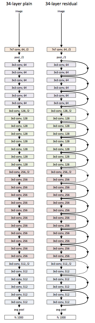Residual Networks

2015 image recognition winner. https://arxiv.org/abs/1512.03385

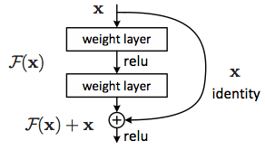
Residual Networks

Residual Networks

Densely Connected Convolutional Neural Networks

https://arxiv.org/pdf/1608.06993.pdf

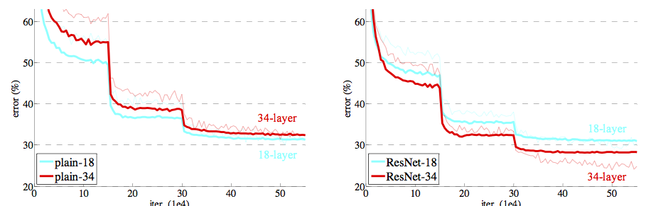
Densely Connected Convolutional Neural Networks

Highway Networks

https://arxiv.org/abs/1505.00387

Like ResNet, but forwarding connections are gated.

• $T$ transform gate - how much of the $H$ transform to keep
• $C$ carry gate - how much of previous input to keep $$y = H(\mathbf{x}, \mathbf{W_T})\cdot T(\mathbf{x}, \mathbf{W_T}) + \mathbf{x} \cdot C(\mathbf{x}, \mathbf{W_T}) \\ C = 1 - T \\ T(\mathbf{x}) = \sigma(\mathbf{W_T}^Tx+\mathbf{b_T}) $$

%%html
<div id="highgate" style="width: 500px"></div>
<script>
$('head').append('<link rel="stylesheet" href="https://bits.csb.pitt.edu/asker.js/themes/asker.default.css" />');

    var divid = '#highgate';
	jQuery(divid).asker({
	    id: divid,
	    question: "Which value for T results in a network most similar to a classical ResNet?",
		answers: ["-1","0","0.5","1","2"],
        server: "https://bits.csb.pitt.edu/asker.js/example/asker.cgi",
		charter: chartmaker})
    
$(".jp-InputArea .o:contains(html)").closest('.jp-InputArea').hide();

</script>

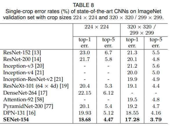
Squeeze and Excitation Networks

https://arxiv.org/pdf/1709.01507.pdf

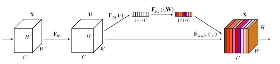
"The features U are first passed through a squeeze operation, which produces a channel descriptor by aggregating feature maps across their spatial dimensions (H × W). The function of this descriptor is to produce an embedding of the global distribution of channel-wise feature responses, allowing information from the global receptive field of the network to be used by all its layers. The aggregation is followed by an excitation operation, which takes the form of a simple self-gating mechanism that takes the embedding as input and produces a collection of per-channel modulation weights."

Squeeze and Excitation

$$F_{sq}(\mathbf{u_c}) = \frac{\sum_i^H \sum_j^W u_c(i,j)}{HW}$$

$$s = F_{ex}(\mathbf{z},\mathbf{W}) = \sigma(\mathbf{W_2} \mathrm{ReLU}(\mathbf{W_1}\mathbf{z}))$$

$$F_{\mathit{scale}}(\mathbf{u_c},s_c) = s_c\mathbf{u_c}$$

Squeeze and Excitation

Things to try for improving a CNN

• Batch norm
• "Network in a network" 1x1 filters
• More layers
• Residual connections
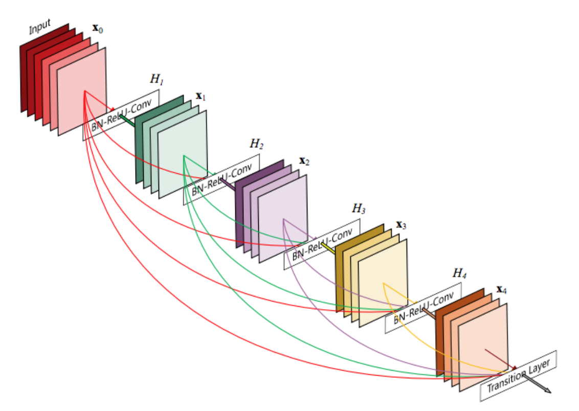
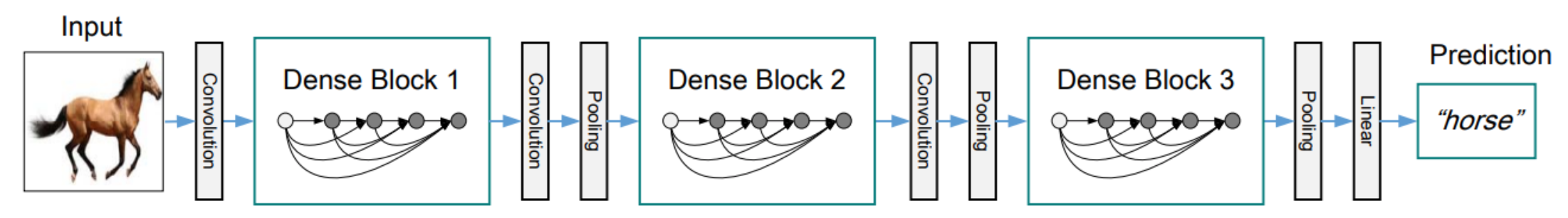
• Dense connections
• Squeeze and Excitation

How would you apply a CNN to DNA sequences?

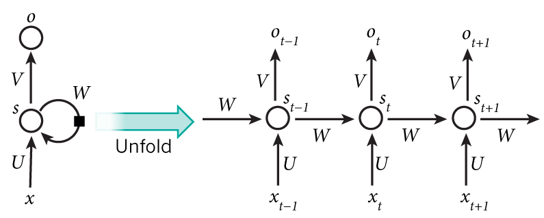
Recurrent Neural Networks

CNNs process spatial relationships. What about temporal? Arbitrary length sequences?

RNNs

https://blog.floydhub.com/a-beginners-guide-on-recurrent-neural-networks-with-pytorch/

RNNs

Many-to-one

RNNs

Many(N) to many(N)

RNNs

Many(N) to many(M)

Sequence-to-sequence

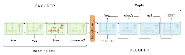
Sequence-to-sequence (Encoder/Decoder)

Decoder uses its own outputs as inputs.

• Teacher-forcing: during training provide correct inputs
• Pros? Cons?

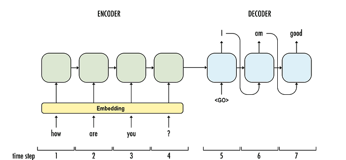
https://towardsdatascience.com/sequence-to-sequence-model-introduction-and-concepts-44d9b41cd42d

What would you use...

• to processes assignment subsequences and predict chromatin accessibility?
• to convert DNA to protein sequence?
• to summarize a research article into an abstract?
• to auto-complete a sequence?

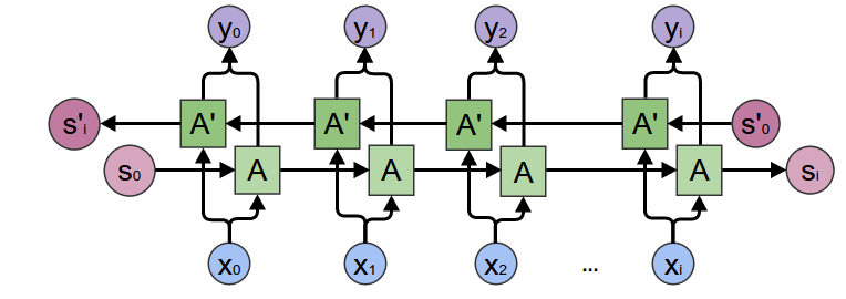
Bidirectional RNN

Normal RNN + RNN going in reverse.

At each point have both forward and backwards context.

http://colah.github.io/posts/2015-09-NN-Types-FP/

RNNs

What is inside these RNN "boxes"?

• A function of the input and some generated "hidden" state(s)
• Can be arbitrarily complex

Gated Recurrent Unit

• $x_{t}$: input vector
• $h_{t}$: output vector
• $z_{t}$: update gate vector
• $r_{t}$: reset gate vector

%%html
<div id="gru" style="width: 500px"></div>
<script>
    var divid = '#gru';
	jQuery(divid).asker({
	    id: divid,
	    question: "Which is a learned parameter?",
		answers: ["x","h","z","b"],
        server: "https://bits.csb.pitt.edu/asker.js/example/asker.cgi",
		charter: chartmaker})
    
$(".jp-InputArea .o:contains(html)").closest('.jp-InputArea').hide();


</script>

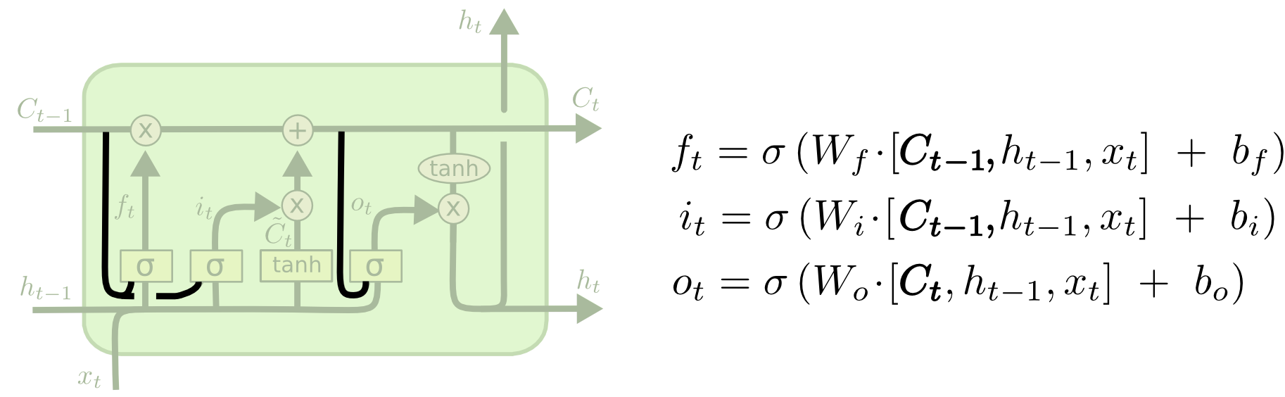
LSTMs

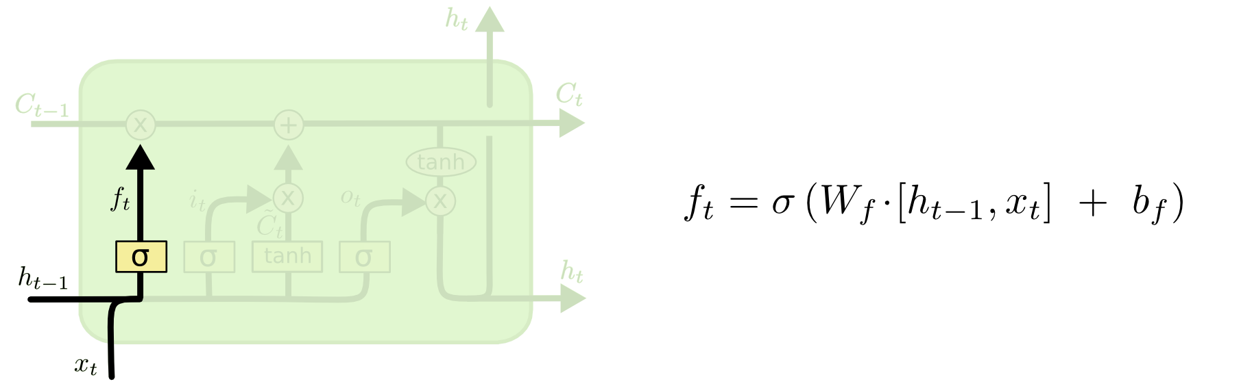
Long short term memory. http://colah.github.io/posts/2015-08-Understanding-LSTMs/

LSTMs maintain a cell state that is seperate from the hidden state.

LSTMs: forget gate

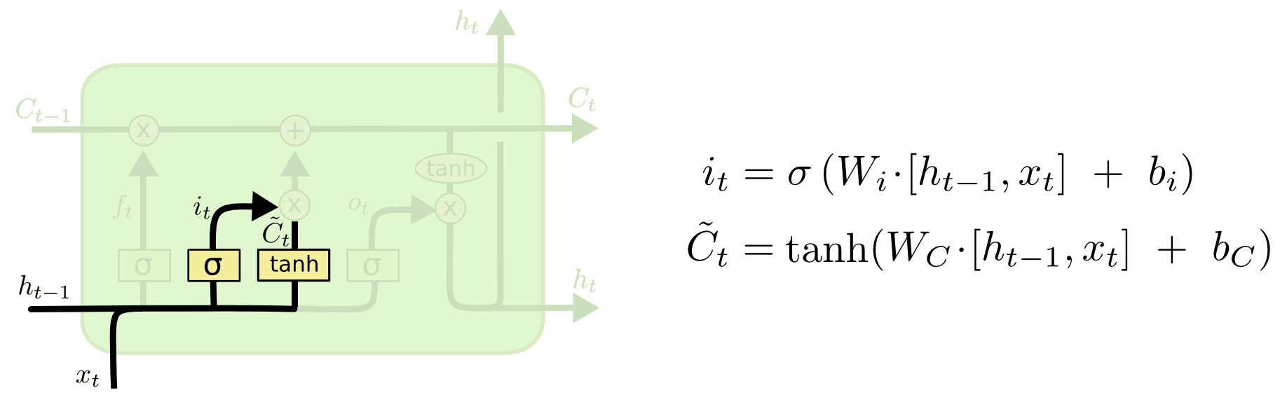
LSTMs: input gate

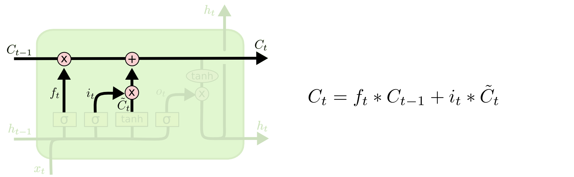
LSTMs: update cell state

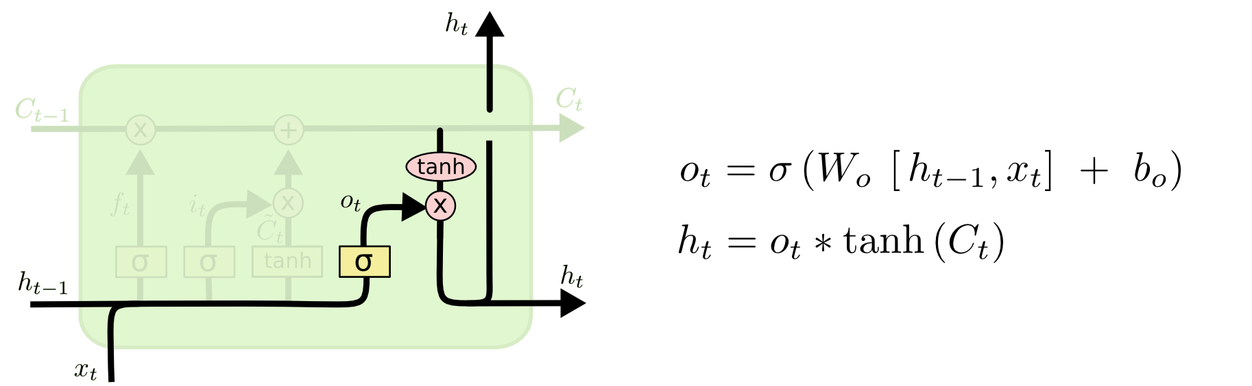
LSTMs: output state

Peephole LSTM

RNNs Writing your email...

https://research.googleblog.com/2015/11/computer-respond-to-this-email.html

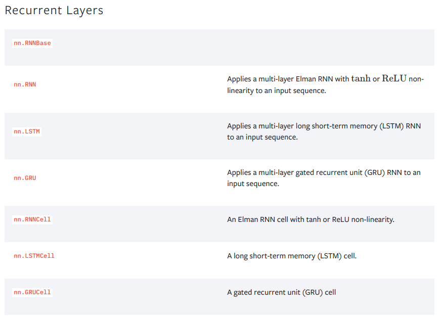
PyTorch RNN

Let's train an RNN on the assignment chromatin accessibility data.

First create a custom dataset.

import torch

class SeqDataset(torch.utils.data.Dataset):
    def __init__(self, fname):
        #process whole file into memory
        self.seqs = []
        self.labels = []
        encodings = {'a': [1,0,0,0],'c': [0,1,0,0], 'g': [0,0,1,0], 't': [0,0,0,1], 'n': [0,0,0,0]}
        for line in open(fname):
            seq,label = line.split()
            self.seqs.append(torch.tensor(list(map(lambda c: encodings[c], seq.lower())),dtype=torch.float32))
            self.labels.append(float(label))        
            
    #a mappable dataset needs __len__ and __getitem__
    def __len__(self):
        return len(self.seqs)
    def __getitem__(self, idx):
        return {'seq':self.seqs[idx], 'label': self.labels[idx]}

%%time
dataset = SeqDataset('train.B.txt')
dataloader = torch.utils.data.DataLoader(dataset, batch_size=20, shuffle=True)

CPU times: user 55 s, sys: 829 ms, total: 55.8 s
Wall time: 56.6 s

Why these timings?

class SeqDataset2(torch.utils.data.Dataset):
    def __init__(self, fname):
        #process whole file into memory
        self.seqs = []
        self.labels = []
        self.encodings = {'a': [1,0,0,0],'c': [0,1,0,0], 'g': [0,0,1,0], 't': [0,0,0,1], 'n': [0,0,0,0]}
        for line in open(fname):
            seq,label = line.split()
            self.seqs.append(seq.lower())
            self.labels.append(float(label))        
            
    #a mappable dataset needs __len__ and __getitem__
    def __len__(self):
        return len(self.seqs)
    def __getitem__(self, idx):
        seq = torch.tensor(list(map(lambda c: self.encodings[c], self.seqs[idx])),dtype=torch.float32)        
        return {'seq':seq, 'label': self.labels[idx]}

%%time
dataset2 = SeqDataset2('train.B.txt')
dataloader2 = torch.utils.data.DataLoader(dataset2, batch_size=20, shuffle=True)

CPU times: user 557 ms, sys: 83.5 ms, total: 640 ms
Wall time: 662 ms

%%time
for batch in dataloader2:
    pass

CPU times: user 56.2 s, sys: 2.42 ms, total: 56.2 s
Wall time: 56.9 s

%%time
dataset2 = SeqDataset2('train.B.txt')
dataloader2 = torch.utils.data.DataLoader(dataset2, batch_size=20, shuffle=True,num_workers=8)

CPU times: user 452 ms, sys: 121 ms, total: 573 ms
Wall time: 497 ms

%%time
for batch in dataloader2:
    pass

CPU times: user 12.8 s, sys: 4.36 s, total: 17.2 s
Wall time: 34.7 s

%%time
for batch in dataloader2:
    pass

CPU times: user 13.1 s, sys: 4.57 s, total: 17.6 s
Wall time: 35.7 s

Pros and cons of lazy loading?

Variable length inputs

Our dataset conveniently has all the same length sequences. If they had different lengths we would have to pad each batch by providing a collate_fn to our data loader.

https://stackoverflow.com/questions/65279115/how-to-use-collate-fn-with-dataloaders

def collate_fn(data):
    """
       data: is a list of tuples with (example, label, length)
             where 'example' is a tensor of arbitrary shape
             and label/length are scalars
    """
    _, labels, lengths = zip(*data)
    max_len = max(lengths)
    n_ftrs = data[0][0].size(1)
    features = torch.zeros((len(data), max_len, n_ftrs))
    labels = torch.tensor(labels)
    lengths = torch.tensor(lengths)

    for i in range(len(data)):
        j, k = data[i][0].size(0), data[i][0].size(1)
        features[i] = torch.cat([data[i][0], torch.zeros((max_len - j, k))])

    return features.float(), labels.long(), lengths.long()

#https://github.com/gabrielloye/RNN-walkthrough/blob/master/main.ipynb
class Model(nn.Module):
    def __init__(self, input_size, output_size, hidden_dim, n_layers):
        super(Model, self).__init__()

        # Defining some parameters
        self.hidden_dim = hidden_dim
        self.n_layers = n_layers

        #Defining the layers
        # RNN Layer
        self.rnn = nn.RNN(input_size, hidden_dim, n_layers, batch_first=True)   
        # Fully connected layer
        self.fc = nn.Linear(hidden_dim, output_size)
    
    def forward(self, x):
        
        batch_size = x.size(0)

        #Initializing hidden state for first input using method defined below
        hidden = self.init_hidden(batch_size)

        # Passing in the input and hidden state into the model and obtaining outputs
        out, hidden = self.rnn(x, hidden)

        # Ignore outputs, compute final value from final hidden state
        out = self.fc(hidden[-1]) # hidden is n_layers * n_directions x batch x hidden_size
        
        return out.flatten()
    
    def init_hidden(self, batch_size):
        # This method generates the first hidden state of zeros which we'll use in the forward pass
        hidden = torch.zeros(self.n_layers, batch_size, self.hidden_dim).to('cuda')
         # We'll send the tensor holding the hidden state to the device we specified earlier as well
        return hidden

When training a CNN, the tensor is usually has the batch size as the first dimension.

When training an RNN, the tensor usually has the timestep as the first dimension and the batch as the second (batch_first defaults to False).

Why?

This can making shaping/slicing output a little tricky: https://pytorch.org/docs/stable/generated/torch.nn.RNN.html#torch.nn.RNN

%%time
model = Model(input_size=4, output_size=1, hidden_dim=256, n_layers=2).to('cuda')
optimizer = torch.optim.Adam(model.parameters(), lr=0.0001)

losses = []
for i,batch in enumerate(dataloader):
    optimizer.zero_grad()
    output = model(batch['seq'].to('cuda'))
    labels = batch['label'].type(torch.float32).to('cuda')
    loss = F.mse_loss(output,labels)
    loss.backward()
    optimizer.step()
    losses.append(loss.item())

CPU times: user 2min 4s, sys: 1.4 s, total: 2min 6s
Wall time: 2min 9s

plt.plot(losses)

[<matplotlib.lines.Line2D at 0x7f38cc3feec0>]

Test Performance

testset = SeqDataset('test.B.labeled.txt')
testloader = torch.utils.data.DataLoader(testset, batch_size=20)

pred = []
true = []
with torch.no_grad():
    for batch in testloader:
        output = model(batch['seq'].to('cuda'))
        true += batch['label']
        pred += output.tolist()

np.corrcoef(pred,true)

array([[1.       , 0.2784861],
       [0.2784861, 1.       ]])

def count_parameters(model):
    return sum(p.numel() for p in model.parameters() if p.requires_grad)

count_parameters(model)

198913

class LSTMModel(nn.Module):
    def __init__(self, input_size, output_size, hidden_dim, n_layers):
        super(LSTMModel, self).__init__()

        # Defining some parameters
        self.hidden_dim = hidden_dim
        self.n_layers = n_layers

        #Defining the layers
        # RNN Layer
        self.lstm = nn.LSTM(input_size, hidden_dim, n_layers, batch_first=True)   
        # Fully connected layer
        self.fc = nn.Linear(hidden_dim, output_size)
    
    def forward(self, x):
        
        batch_size = x.size(0)

        #Initializing hidden state for first input using method defined below
        hiddenc = self.init_hidden(batch_size)

        # Passing in the input and hidden state into the model and obtaining outputs
        out, hiddenc = self.lstm(x, hiddenc)

        # Ignore outputs, compute final value from final hidden state
        out = self.fc(hiddenc[0])
        
        return out.flatten()
    
    def init_hidden(self, batch_size):
        # Both the hidden and cell state
        hiddenc = (torch.zeros(self.n_layers, batch_size, self.hidden_dim).to('cuda'),
                    torch.zeros(self.n_layers, batch_size, self.hidden_dim).to('cuda'))
         # We'll send the tensor holding the hidden state to the device we specified earlier as well
        return hiddenc

%%time
model = LSTMModel(input_size=4, output_size=1, hidden_dim=256, n_layers=1).to('cuda')
optimizer = torch.optim.Adam(model.parameters(), lr=0.0001)

losses = []
for i,batch in enumerate(dataloader):
    optimizer.zero_grad()
    output = model(batch['seq'].to('cuda'))
    labels = batch['label'].type(torch.float32).to('cuda')
    loss = F.mse_loss(output,labels)
    loss.backward()
    optimizer.step()
    losses.append(loss.item())

CPU times: user 4min 36s, sys: 943 ms, total: 4min 37s
Wall time: 4min 40s

plt.plot(losses)

[<matplotlib.lines.Line2D at 0x7f38cccf29b0>]

pred = []
true = []
with torch.no_grad():
    for batch in testloader:
        output = model(batch['seq'].to('cuda'))
        true += batch['label']
        pred += output.tolist()

np.corrcoef(pred,true)

array([[1.        , 0.20315939],
       [0.20315939, 1.        ]])

count_parameters(model)

268545

Further improving this is left as an exercise for the reader

Quiz